Authored by Wang, Chen and Kim
The bike-sharing service has brought many conveniences to citizens and served as an effective supplement to mass transit system. For docked bike-sharing service, each docking station has the fixed spots to store bikes and stations could be empty or saturated at some time. Bike-sharing operators would redistribute bikes between stations by trucks according to their experiences. It is ineffective for the operation and inconvenient for users to access this service smoothly. There are many studies on short-term forecasting in transportation, such as traffic flow, traffic congestion, traffic speed, passenger flow and more. However, their applications in the field of bike-sharing still remain blank. This paper mainly focuses on the short-term forecasting for docking station usage in a case of Suzhou, China. The widely used methodologies in forecasting are reviewed and compared. After that, two latest and highly efficient models, LSTM and GRU, are adopted to predict the short-term available number of bikes in docking stations with one-month historical data. RF is used to be compered as a benchmark. The predicted results show that LSTM and GRU which derive from RNN and Random Forest achieve good performance with acceptable error and comparative accuracies. Random forest is more advantageous in terms of training time while LSTM with various structures can predict better for long term. The maximum difference between the real data and predicted value is only 1 or 2 bikes, which supports the developed models are practically ready to use.

FIGURE 2 Locations of the stations.
LSTM
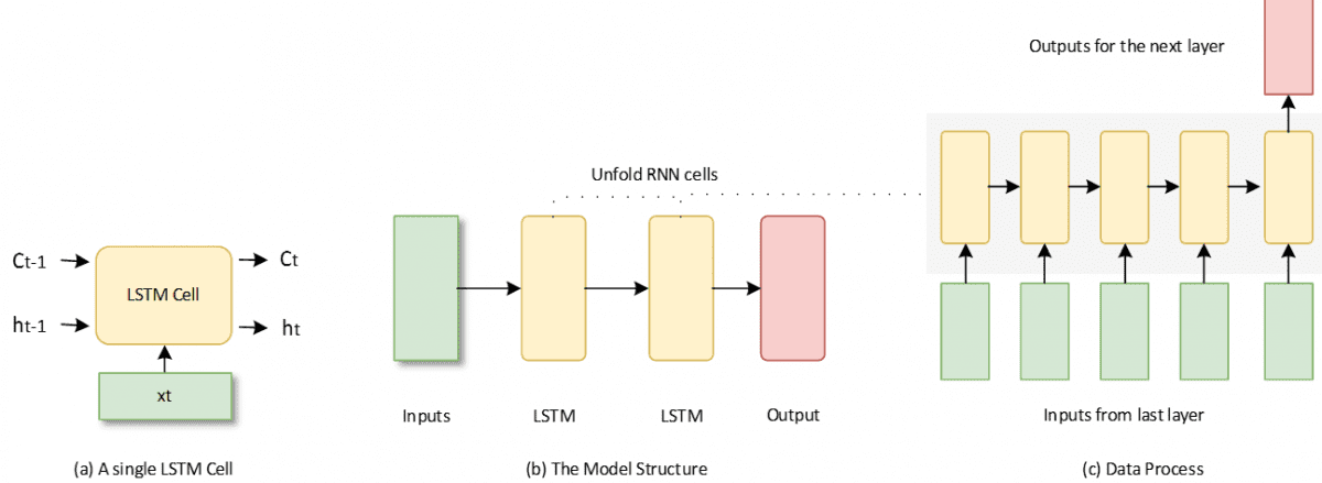
The Long short-term memory neural networks (LSTM) is a special kind of recurrent neural networks for the time series prediction (28). As shown in the Figure 4 (a), the LSTM cell can hold and update a state during the training process. Thus, the model makes a prediction with the previous learning experience. The mathematical expressions can be denoted as
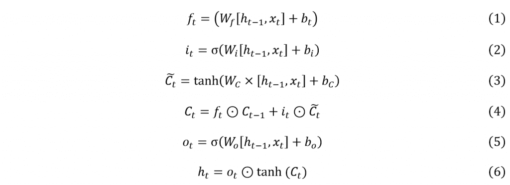
where is the current step, is the input, is the output, is the weight matrix, is the bias. , , and are intermediate variables, which decide to remember or forget the input data (29).
Two LSTM layers are used in this paper and the output layer would make a final regression results. Figure 4 (b) shows basic structure of the model as well as the running steps of the LSTM cells. When the continuous input values flow in the LSTM cell, it will unfold and handle these values by sequence as figure 4 (c). After the last one is finished, the cell would make an output result for the next layer.

FIGURE 4 Description of the LSTM model.
GRU
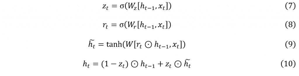
Gated Recurrent Unit (GRU) was introduced in 2014 (30). It’s an improved recurrent neural network based on LSTM. It merges the input part and forgetting part together so the number of the gates from 4 becomes 3. As a result, GRU saves more computational resources than LSTM with similar performance. To compare the difference between LSTM and GRU, we use same network structure as LSTM in figure 3 (b). The main expressions can be indicated by following formulas (29).
The article used LSTM, GRU and Random Forest with a different time interval and sequence length to predict the number of available bikes. A laptop (Windows 10, 16GB RAM, Intel i7-4720HQ, GeForce GTX 960M) completed the whole training tasks. The LSTM and GRU run on top of Keras (31) and Tensorflow (32)with GPU. For the random forest part, it is coded and run with Scikit-learn (33) and CPU.
| Time Interval | Sequence Length | Training Time (s) – 25 epochs | Training Time (s) – 1000 estimators | |
| LSTM | GRU | RF | ||
| 1 | 5 | 45.83 | 37.59 | 5.31 |
| 10 | 78.15 | 61.58 | 13.62 | |
| 20 | 143.42 | 109.05 | 36.78 | |
| 30 | 210.45 | 160.81 | 64.77 | |
| 5 | 5 | 14.50 | 12.08 | 2.56 |
| 10 | 20.81 | 16.90 | 4.35 | |
| 20 | 34.47 | 26.22 | 8.75 | |
| 30 | 47.81 | 37.37 | 13.71 | |
| 10 | 5 | 10.82 | 6.46 | 1.87 |
| 10 | 13.84 | 7.45 | 2.93 | |
| 20 | 20.97 | 9.68 | 5.32 | |
| 30 | 28.19 | 11.73 | 7.69 | |
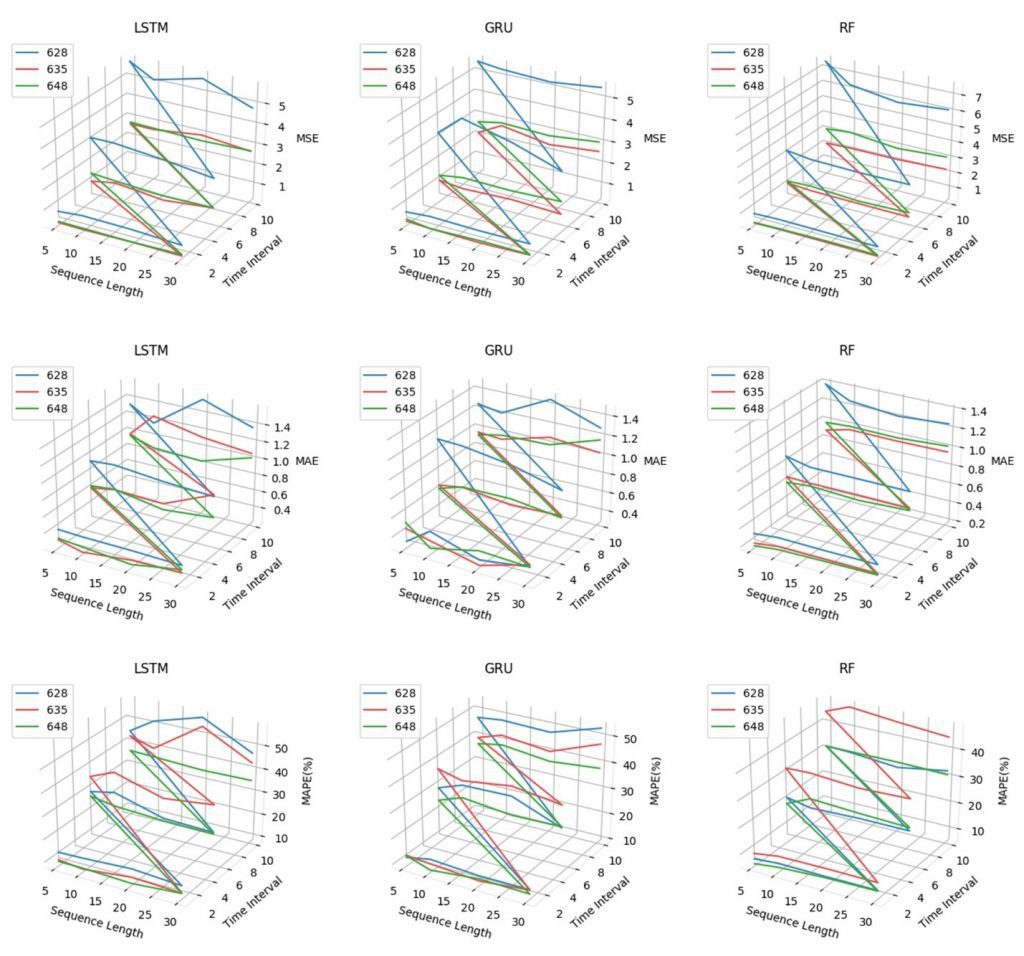
The time interval only has three different levels: 1min, 5mins, and 10mins. Also, the sequence length has four different levels: 5, 10, 20, and 30. As a result, the lines in the graphs are not smooth but broken lines. The main features of these graphs are listed as follows.
- The MSE of RF is very good when the time interval is short but with the increase of the time interval, RF gets worse performance than other two. The memory unit in the RNN may help with long interval sequence;
- Generally, the results are quite similar with these three models. However, the blue line always higher than others in the graph of GRU and Random Forest, which means station 628 get worse results in those two models. Since 628 station has the larger usage amount, the variation may be higher than others;
- All lines get higher with the increase of the time interval. There are two potential reasons may cause this problem. One is that forecasting long time interval is harder. The other one is that the sample size is dramatically decreased when expanding the interval so that the accuracy is affected;
- Different sequence lengths do not change much performance of models but sequence lengths affect the results gently and the longer one leads to a better performance in most cases.
- LSTM, GRU and Random Forest are all following the trends very well. The difference between the real data and predicted data is less than 1 or 2 bikes. It is good enough to help to develop the bike-sharing management based on these predictions;
- The accuracies between the three predictions are very comparative;
- LSTM and GRU get similar trends in most of the cases because they might have similar model structures;
- When the time interval is short, random forest gets a better performance;
- By increasing the sequence length, the fluctuation of three predictions is

Comments are closed.