Imputation of Missing data

INTRODUCTION

Transportation data is of great importance for intelligent transportation system. Missing data problems are inevitable during data collection.

Challenges in existing imputation methods: potential useful information is not efficiently used in the modeling process; methods considering temporal correlation usually assuming that linear relationships exist between observed variables and latent variables; most techniques fail to measure the uncertainty.

This study introduces the use of a self-measuring multi-task Gaussian process (SM-MTGP) method for imputing missing data.

CONTRIBUTIONS

A SM-MTGP method is proposed to combine features from tasks and inputs to measure similarities jointly.

Dependencies of tasks and inputs are explored via covariance functions under SM-MTGP framework.

Correlations between responses are captured to provide additional information for enhancing imputation accuracy.

METHODOLOGY

Brief review of MTGP

Assuming we have $Q$ tasks and a set of observations $Y = \left\{ {{y_{i1}},{y_{i2}}, \ldots {y_{iD}}} \right\}, i = 1, \ldots ,Q$, for each corresponding task at $????$ distinct inputs, where $????_{????????}$ is the response for $????^{????ℎ}$ task given the input $????_????$.

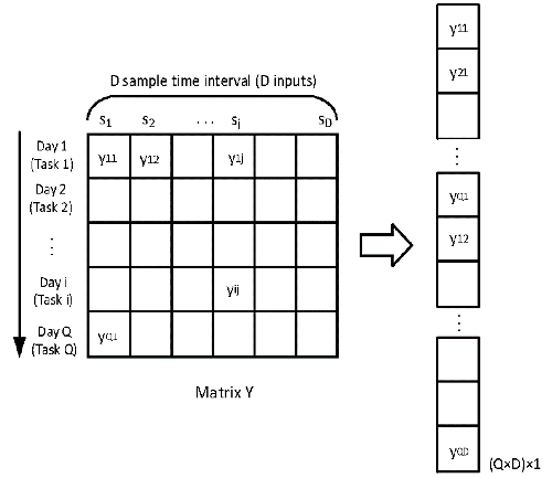
FIGURE 1 Vectorization of matrix Y

When the SM-MTGP model is introduced to the imputation of missing values of transfer passenger flow, the shared information of tasks is considered in terms of the temporal relatedness of various days. Transfer passenger flow over $Q$ days can be treated as $Q$ tasks, and the number of sampling time intervals $D$ per day represents $D$ distinct inputs. We define a matrix $Y = \left\{ {{y_{ij}}} \right\}(i = 1,2,…,Q;j = 1,2,…D) \in Q \times D $, where ${{y_{ij}}}$ is number of transfer passengers for the ${i^{th}}$ day (task) on the ${j^{th}}$ time interval (input). By stacking the column vectors of $Y \in Q \times D $, a $Q \times D$ dimension vector ${\bf{y}} = vec(Y)$ is obtained (Figure 1).

The MTGP model of ${{\bf{\tilde y}}}$can be described as Equation (1):
$${{\tilde y}_{ij}} = {m_{ij}} + \varepsilon ,\quad \varepsilon \sim N\left( {0,{\sigma ^2}} \right) \tag{1}$$ where ${m_{ij}}$ is the expected value of the element ${{\tilde y}_{ij}}$, and $\varepsilon$ is an additive Gaussian noise with variance ${{\sigma ^2}}$.
$$m \sim N\left( {0,{\Sigma _Q} \otimes {\Sigma _D}} \right) \label{TGP} \tag{2}$$ $${\Sigma _Q} = K_Q^fG_Q^m, \quad{\Sigma _D} = K_D^fG_D^m \label{covariance matrix} \tag{3}$$ The covariance matrices ${\Sigma _Q}$ are defined as a product of kernel of days features (tasks) $K_Q^f$ and the self-measuring kernel $G_Q^m$, and ${\Sigma _D}$ are defined as a product of the kernel of time intervals features (inputs) $K_D^f$ and self-measuring kernel $G_D^m$.
$${K_Q^f} = k\left( {{y_i},{y_j}} \right) \in \mathbb{R}^{Q \times Q}, \quad {G_Q^m} = g\left( {{y_{i:}},{y_{j:}}} \right) \in \mathbb{R}^{Q \times Q} \tag{4}$$ $${K_D^f} = k\left( {{y_h},{y_l}} \right) \in \mathbb{R}^{D \times D}, \quad {G_D^m} = g\left( {{y_{:h}},{y_{:l}}} \right) \in \mathbb{R}^{D \times D} \tag{5}$$ where $k\left( {{y_i},{y_j}} \right)$ and $k\left( {{y_h},{y_l}} \right)$ indicate covariances of features of ${i^{th}}$ day and ${j^{th}}$ day, and covariances of features of ${h^{th}}$ time interval and ${l^{th}}$ time interval, respectively. Similarly, $g\left( {{y_{i:}},{y_{j:}}} \right)$ and $g\left( {{y_{:h}},{y_{:l}}} \right)$ measure covariances of self-measuring observations of ${i^{th}}$ day and ${j^{th}}$ day, and covariances of self-measuring observations of ${h^{th}}$ time interval and ${l^{th}}$ time interval.

By following the principle of MTGP, the joint distribution of ${\tilde Y}$ can be described as Equation (6), where $\Phi = {\Sigma _Q} \otimes {\Sigma _D} + {\sigma ^2}{\bf{I}}$.
$$\int {p\left( {\tilde Y|M,0,{\sigma ^2}} \right)} p\left( {M|{\Sigma _Q},{\Sigma _D}} \right)dM = N\left( {{\bf{\tilde y}}|{\bf{0}},\Phi } \right) \tag{6}$$ Using a Gussian process framework given the observed number of transfer passengers, the unobserved passenger flows in $Y$ can be derived by predictive equation (7). $$E[{{\tilde y}_{ab}}|{{{\bf{\tilde y}}}_{obs}},{\Sigma _Q},{\Sigma _D}] = \left( {{\Sigma _{{Q_a}}} \otimes {K_{{D_b}}}} \right)_{obs}^T\Phi _{obs}^{ – 1}{{{\bf{\tilde y}}}_{obs}} \tag{7}$$ where ${\Phi _{obs}} = {\bf{P}}\Phi {{\bf{P}}^T} \in \mathbb{R}^{M \times M} $ is a covariance matrix over the observed transfer passenger flows in $Y$, ${{\Sigma _{{Q_a}}}}$ denotes ${a^{th}}$ column vector in ${\Sigma _Q}$, which measures the similarities between ${a^{th}}$ day and all the other days among $Q$ days, and ${{K_{{D_b}}}}$ indicates ${b^{th}}$ column vector of ${K_D}$, which represents covariance between ${b^{th}}$ time interval and all the remaining time intervals of $D$ samples.

EXPERIMENT

Data analysed includes 6-months of passenger flow data collected by WiFi sensors at Richmond railway station (Figure 2), Melbourne, Australia.

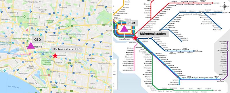
FIGURE 2 Map of location and train lines of Richmond station.

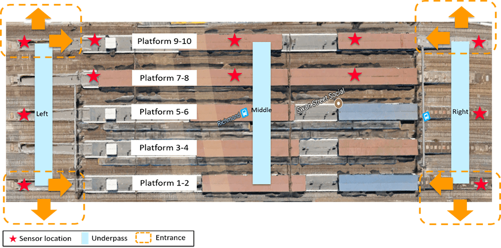
FIGURE 3 Map of 12 WiFi sensors distribution.

The deployed 12 sensors are distributed at platforms 7-10 and two sided underpasses (Figure 3).

IMPUTATION PERFORMANCE

Figure 4 indicates the RMSE results of discrete missing pattern with various algorithms. The improvements in RMSE by SM-MTGP is around 60% for three different missing rates.

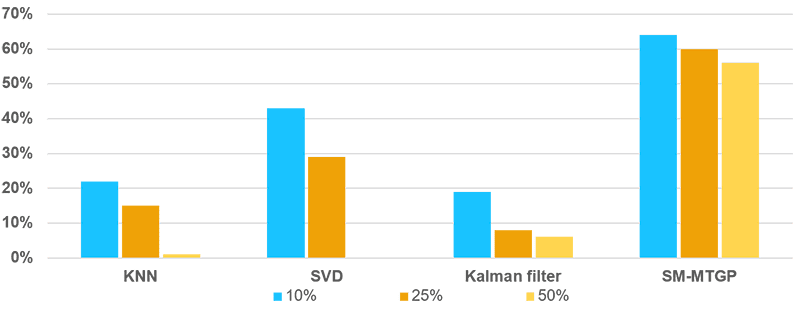
FIGURE 4 RMSE Results for Different Missing Ratios of Discrete missing data.

Three mixed missing patterns under different missing ratios are reported (Figure 5-7). The SM-MTGP method is still able to obtain better performance compared with all the other methods, leading to improvements in RMSE up to 60%.

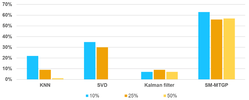
FIGURE 5 RMSE Results for Different Missing Ratios of Mixed Missing Data
with One Random Day Missing.

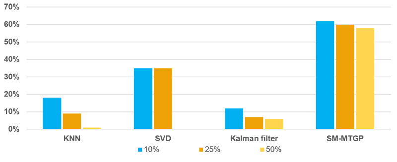
FIGURE 6 RMSE Results for Different Missing Ratios of Mixed Missing Data
with Two Random Day Missing.

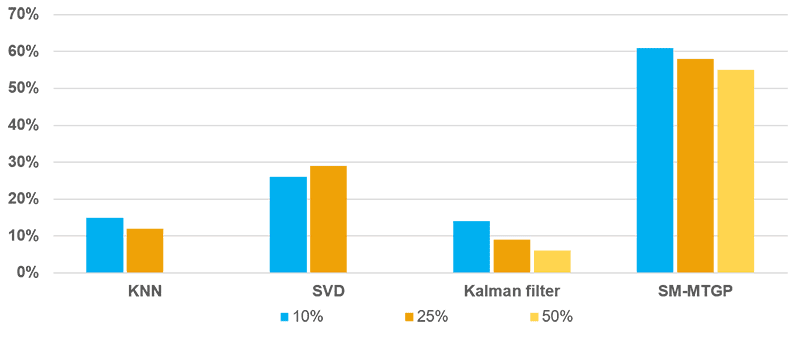
FIGURE 7 RMSE Results for Different Missing Ratios of Mixed Missing Data
with Four Random Day Missing.

CONCLUSIONS

Imputation accuracy can achieve around 60% improvement in RMSE in all the tested missing scenarios compared with the base model.

SM-MTGP significantly outperforms other methods under the large missing ratio.

On-going research on incorporating other features into this algorithm to make application on large-scale transit network and simplifying model computational complexity.

For more detailed information please contact our TUPA members below;
Wenhua Jiang, [email protected]