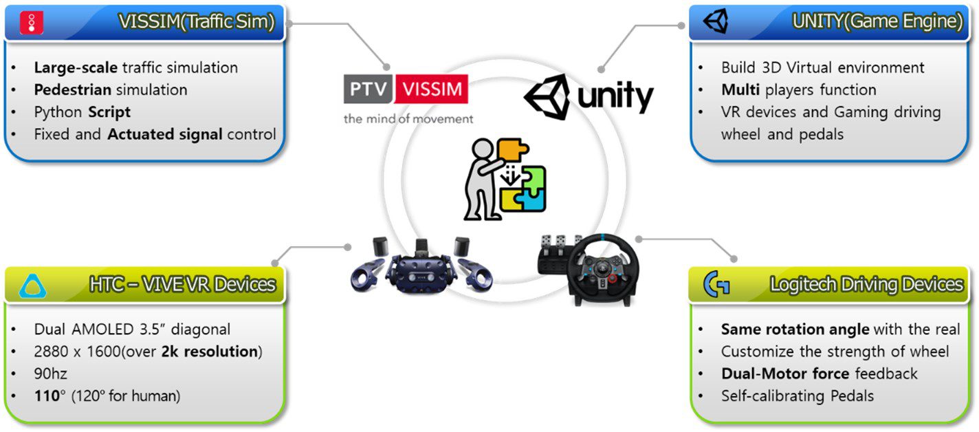
Unity-Vissim Cosimulation environment development for Human-in-the-loop test
Existing human-in-the-loop (HIL) test systems have limitations in providing a realistic traffic environment.
Microsimulation(VISSIM) is mainly used for traffic flow analysis because it embeds models that reflect general human driving behaviors(such as car-following and lane change).
By integrating the two software, the cosimulation environment was built to analyze driving behaviors in realistically reproduced traffic flow situations.
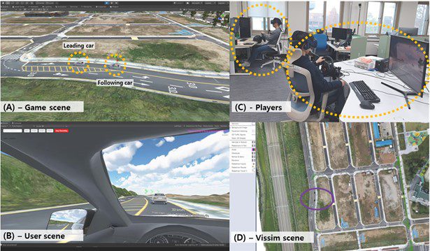
Networking based Multiagent driving simulator platform development
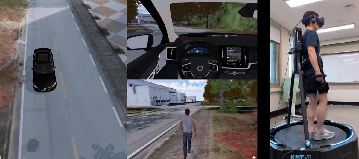
Single Driving simulator has limitations in accurately reflecting human factors in collision risk situations, as vehicles in the simulation operate based on specific models.
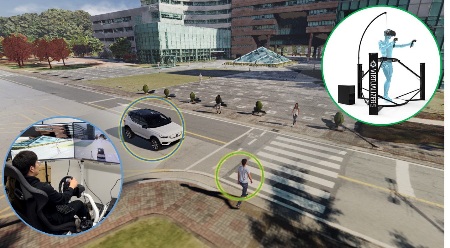
To overcome the limitations, a network-based multiagent driving simulator platform was developed, enabling multiple participants to engage simultaneously.
To verify the reliability of the simulator, scenarios such as car following and unsignalized intersection crossing were selected. Real-world coordinates and speed changes were collected and statistically analyzed alongside corresponding data gathered from the simulators.
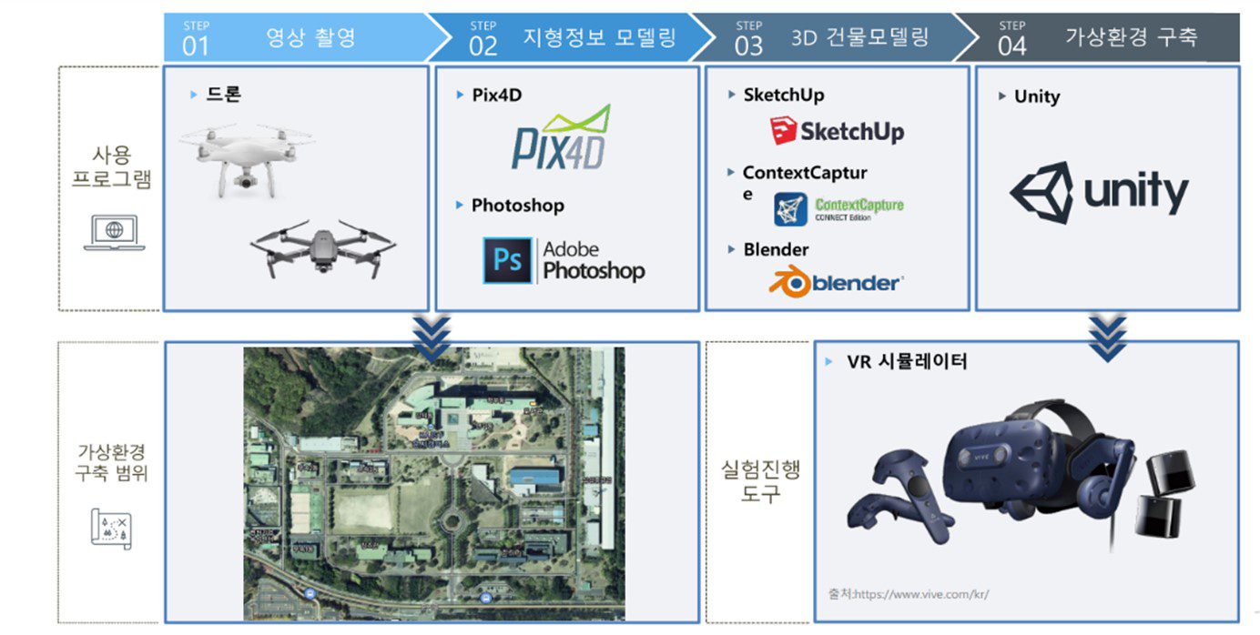
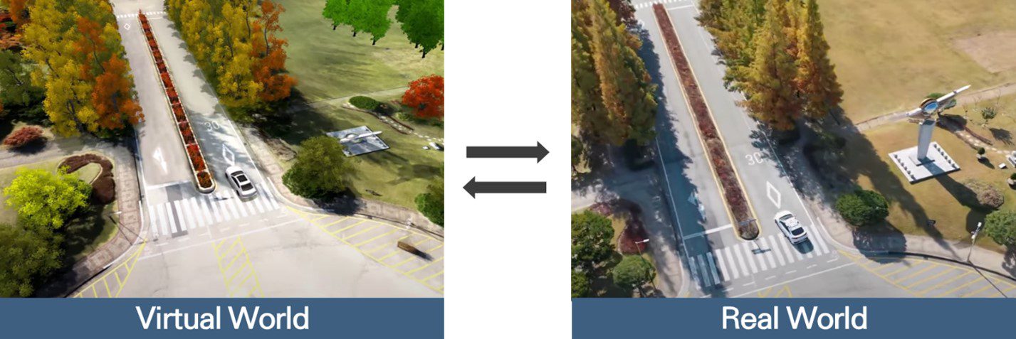
KAIST Munji campus testbed transplantation to the virtual world
To conduct a test-based study, the KAIST Munji campus was scanned using a drone.
Point cloud data was collected and used for 3D modeling.
Performed autonomous vehicle data replay in the metaverse environment based on the trajectory provided in Prof. Dongseok Kum’s laboratory (VDC lab).
Pedestrian model control module was embedded into the developed multiagent simulator platform to extend vehicle-human interactions cases.
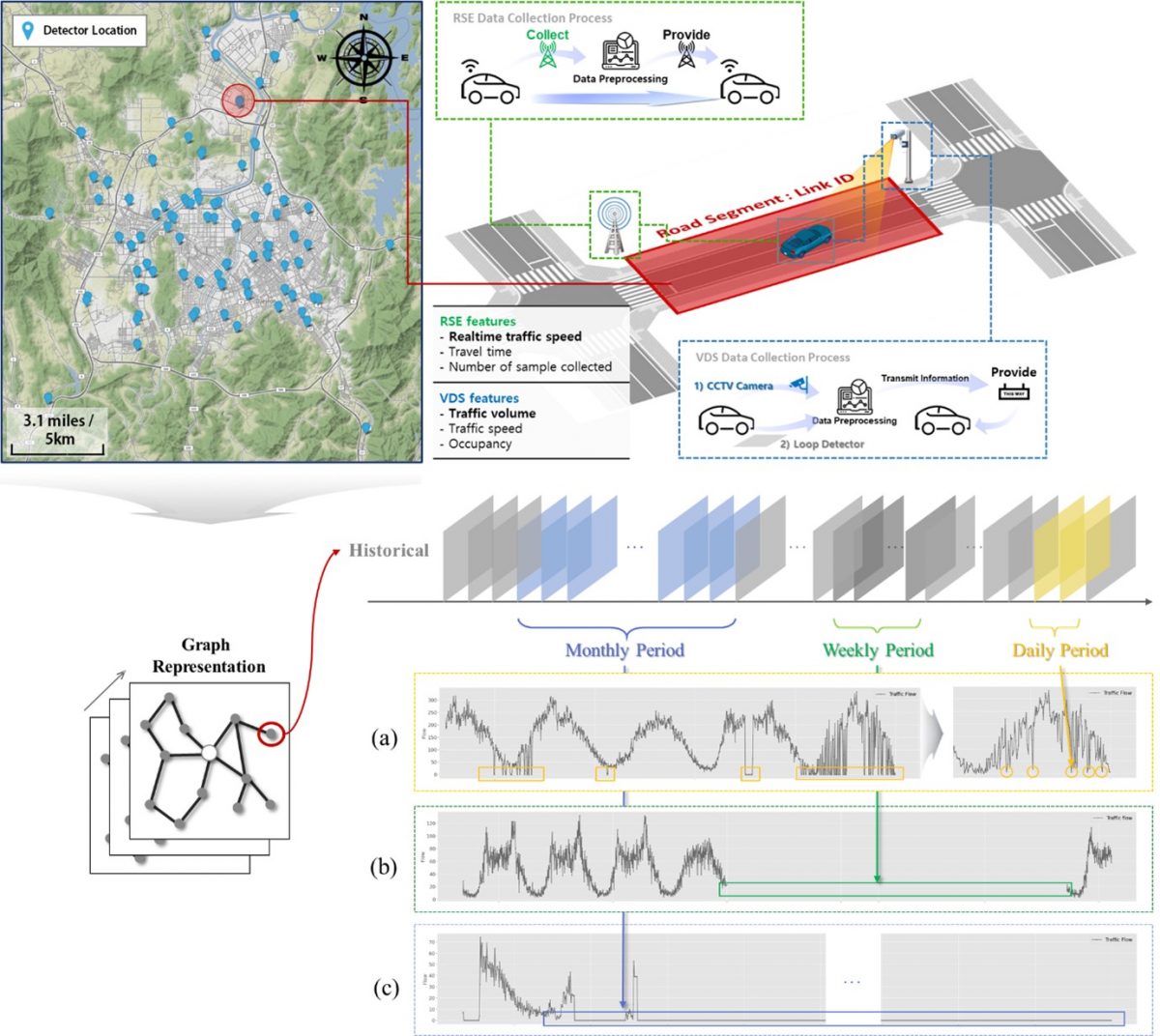
Traffic volume imputation based on multi-source data collection system
Traffic detectors collect traffic data to understand the flow of traffic on a city scale, which can help build an efficient traffic management system or deliver useful traffic information to road users for better decision-making.
However, various types of missing data occur depending on the data management system and unexpected situations on the road. In the short term, we found that the gaps were hourly, but in the long term, they were monthly.
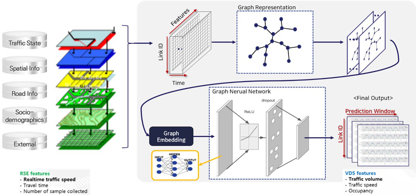
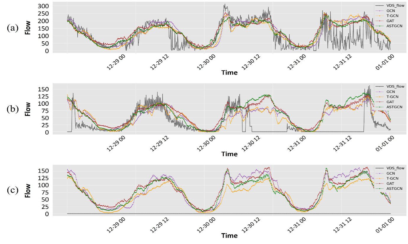
We propose a deep learning methodology based on a graph neural network that can simultaneously interpolate the missing values of a large amount of traffic detector data installed at the city level.
By applying an attention mechanism in the graph domain to cooperatively consider the spatial and temporal correlation of two different types of detectors, the model recovers the original traffic data with an error of less than 12 cars/5 minutes, regardless of the missing data rate.
→ The overall multi-source data aggregation process and imputation procedure
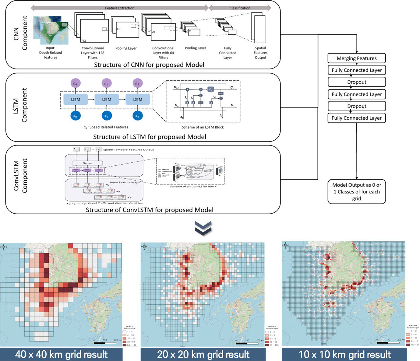
A deep spatio-temporal approach in maritime accident prediction – Predicting the risk of maritime accidents is crucial for improving traffic surveillance and marine safety.
This study aims at investigating the application of deep learning in both short- and long-term predictions of different types of accident risks associated with small vessels by considering multiple influencing factors.
The results reveal that although the performance of the proposed deep spatiotemporal ocean accident prediction (DSTOAP) model varies according to grid sizes and time intervals, its accuracy (more than 78%) makes it reliable for predicting accidents.
Furthermore, although all types of accidents are captured with high accuracy, more than 84% of collision accidents can be predicted accurately.
→ The proposed DSTOAP architecture and prediction results for each grid size
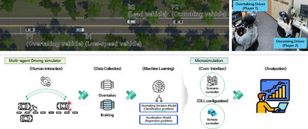
Interactive driving behavior in overtaking situation
Existing studies on overtaking behavior have only examined it from the perspective of the overtaking vehicle, with limited consideration for the risk level of the vehicle approaching from the opposite side.
The multiagent simulator helped collect a realistic overtaking driving dataset without compromising safety. The collected data was preprocessed using SMOTE_Tomek-based imbalanced data techniques to build a high-quality dataset and model human decision-making based on machine learning
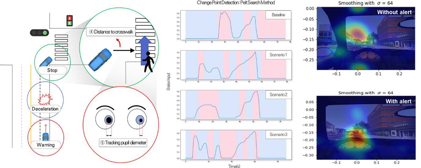
Human Recognition based on ITS technology
Changes in drivers’ cognitive responses and driving behavior were observed when warning right-turning vehicles to improve pedestrian safety at intersections.
By considering human factors such as the driver’s pupil size, viewing position, braking, and acceleration, the points where changes in driving behavior were detected and differences in behavior based on the warning method were analyzed.
Pedestrian behavior
A pedestrian treadmill simulator is connected to the Metaverse simulator platform to calculate parameters for pedestrian height and stride length, ensuring reliable data collection for pedestrians.
This research is to integrate communication, traffic and driver behaviours, vehicle dynamics, and environment conditions in a unison framework to increase safety, reliability, and performance of connected and automated vehicles within a mix traffic condition.
To achieve this goal, TUPA has been developing an architecture that leverages existing tools like VISSIM, Driving simulator, Virtual Reality and Python to analyze and simulate multiple aspects of traffic including vehicles and pedestrians. This tool will enable to develop and validate techniques to improve traffic congestion, safety, and network performance.
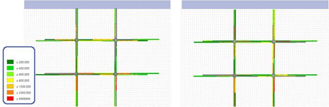
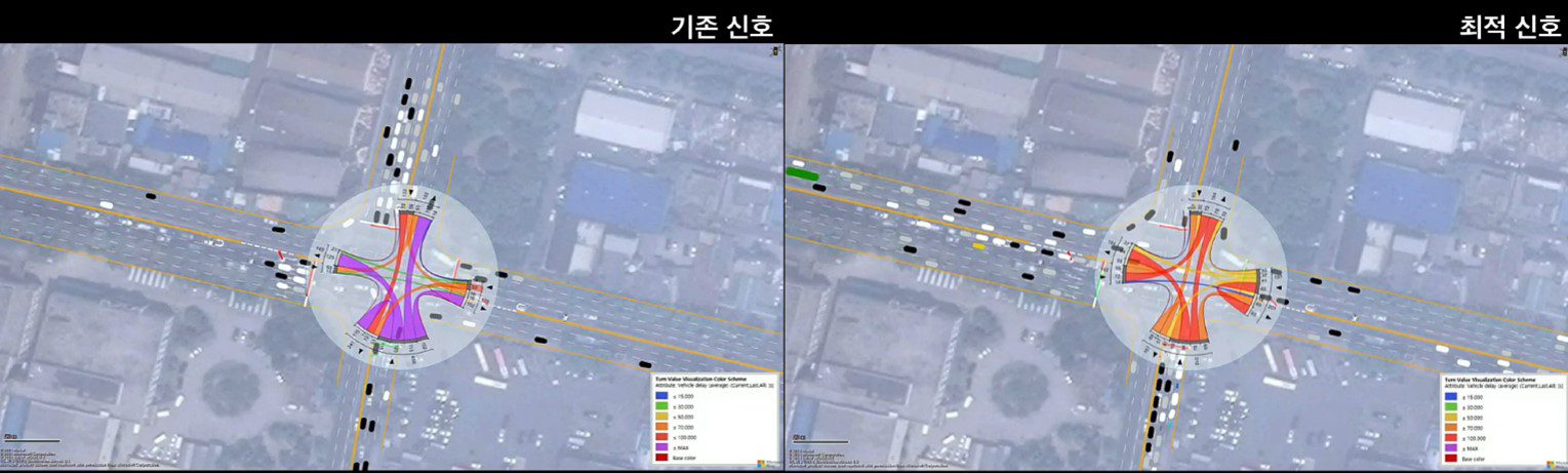
In designing scenarios for the integration of Vissim and Driving simulator, a robust algorithm has been successfully implemented in the platform. This algorithm adapts its behaviour (traffic flow in transport) autonomously in response to the variation of network conditions.
Having human in the loop setting, alternative route guidance information will be displayed in driving simulator so that driver’s decision if he or she is willing to change the route based on the information will be recorded. In this process, the subject vehicle in the simulator and surrounding traffic in VISSIM will interact each other. In addition, all recoded outcomes from the driving simulator will be input to traffic simulation for the large network evaluation. The developed traffic simulation will identify typical traffic indicators such as delay and extreme delay, queue and the number of stops based on the scenarios developed in the driving simulator.
This research keeps developing with the KAIST team since middle of 2019. Transportation experts are aware that it is urgent to take measures to cope with mixed traffic between autonomous vehicles and conventional vehicles, which will be indispensable in the future. It is expected that this new traffic flow not only directly and indirectly leads to traffic accidents but also has a serious side effect on traffic efficiency. Until a fully autonomous vehicle occupies the road, new traffic control techniques are needed. In this study, we propose a new traffic signal controller that supports autonomous driving by driving the driver safely through the virtual environment. This study is expected to be synergistic effect of performance evaluation for future traffic in conjunction with the Connected ITS project and the K-City autonomous vehicle test bed currently underway in Korea. It is expected that many universities and research institutes will benefit from this research since Korea has not developed a human participatory machine learning platform using virtual reality or is in the very early stage.
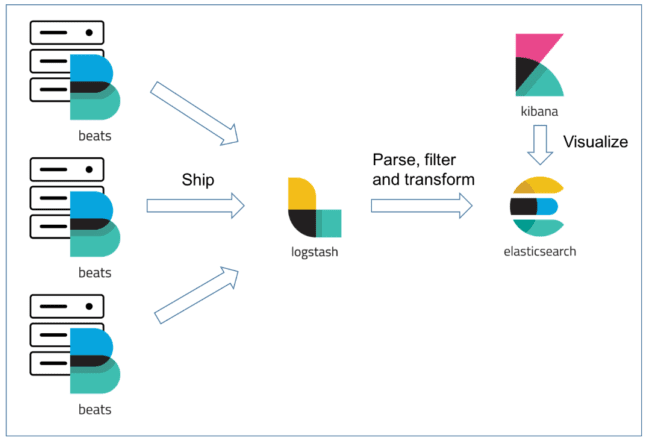
The dashboard below was developed through Elastic open source software using the Seoul metro passenger flow data in 2014.
Data visualization has been important in democratizing data and analytics and making data-driven insights available to workers throughout an organization. Data visualization also plays an important role in big data and advanced analytics projects. As a transportation field accumulated massive troves of data during the early years of the big data trend, they needed a way to quickly and easily get an overview of their data. Visualization tools were a natural fit.
Visualization is central to advanced analytics for similar reasons. When advanced predictive analytics or machine learning algorithms are available, it becomes important to visualize the outputs to monitor results and ensure that models are performing as intended. This is because visualizations of complex algorithms are generally easier to interpret than numerical outputs.
In TUPA, we utilized one of the strongest searching engines called Elasticsearch to make this visualization works. The flowchart below shows the process to deal with big data and visualize it.
We utilized TurtleBot3 which adopts ROBOTIS smart actuator Dynamixel for driving.
TurtleBot3 is a ROS-based mobile robot. We customized it to reconstruct the mechanical parts and use optional parts such as the computer and sensor. SLAM, Navigation and Manipulation, makes it to build a map and can drive around the room. Also, it can be controlled remotely from a laptop, joypad or Android-based smart phone.
The project allows the robot to detect the lane(s) and obstacles to avoid. Various algorithms such as SLAM, CNN, LSTM and OpenManipulator are embedded in the robot to make better robot behavior.
The following video demonstrates the navigation function.
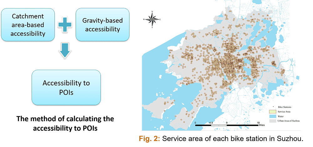
To provide empirical evidence on the relationship between built environment and public sharing bike flow in Suzhou, China.
Research Objectives
To examine the global impacts of built environment on public sharing bike flow.
To understand the effects of spatial variation of those built environment on public sharing bike flow
Study Area
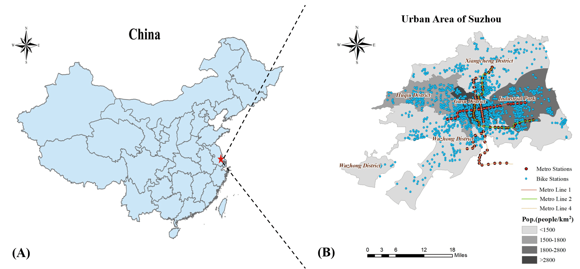
The study area of this research focuses on Suzhou located in the southeast Jiangsu Province of East China and east about 100 km to Shanghai (Figure 1(A)).
There are around 1,750 bike stations and 40,000 public sharing bikes put into use in Suzhou (Figure 1(B)).
Fig. 1: Study area. (A) Location of Suzhou in China; and (B) the spatial distribution of bike stations, metro stations and population density in urban area of Suzhou.
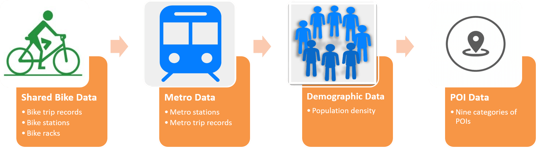
Data
Data Sources
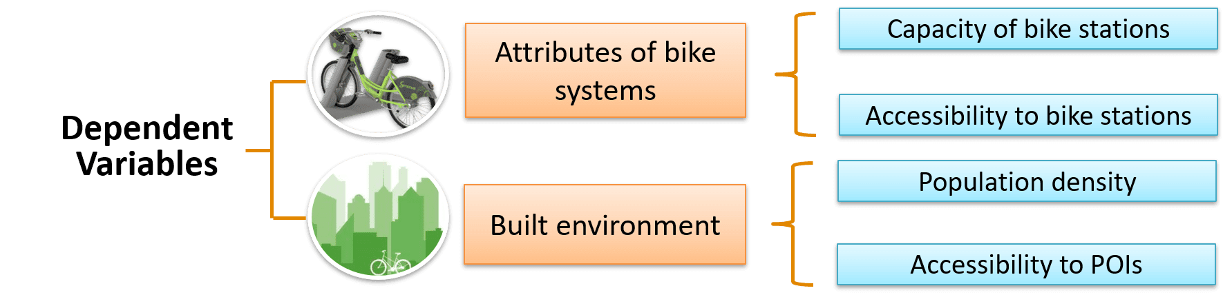
Operationalization of Variables
Methodology
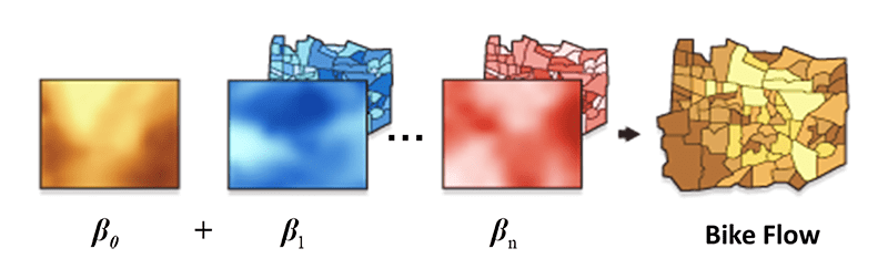
Global Regression
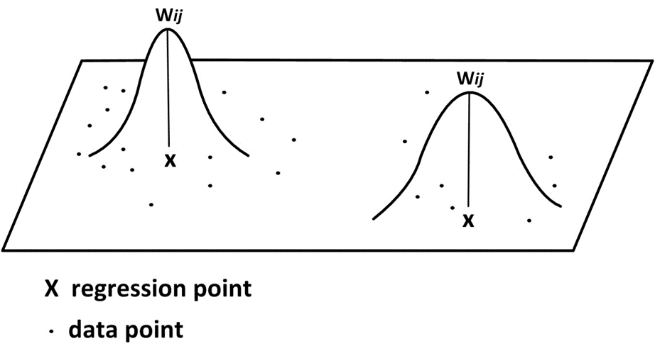
Geographically Weighted Regression (GWR)
GWR is a local regression model. Coefficients are allowed to vary.
Bi-squared Weighting Function
Results and discussions
Global Regression
Table 1: The results of Global Regression.
Dependent variables
Global Regression
Trips on workdays
Trips on nonwork days
Coeff. (t-value)
Coeff. (t-value)
Intercept
-75.388 (-8.27)
-67.948 (-7.25)
Attributes of public bike systems
Capacity of bike stations
3.508 (11.88)
3.372 (11.11)
Accessibility to bike stations
33.441 (14.66)
27.991 (11.93)
Built environment
Population density
-2.2E-04 (-2.13)
-2.2E-04 (-2.00)
Accessibility to metro station
4.852 (5.83)
3.803 (4.44)
Accessibility to shopping mall
8.254 (4.23)
10.003 (4.99)
Accessibility to bus station
6.719 (3.23)
6.054 (2.83)
Accessibility to restaurant
1.075 (5.82)
1.491 (7.84)
Accessibility to dwelling
0.544 (0.49)
0.411 (0.36)
Accessibility to local financial services
11.608 (6.84)
11.494 (6.59)
Accessibility to public leisure and religion place
-3.258 (-2.22)
-0.906 (-0.60)
Accessibility to public park
-7.613 (-1.22)
-1.131 (-0.18)
Accessibility to educational place
7.276 (3.83)
9.130 (4.68)
Accessibility to workplace
5.190 (3.78)
-1.610 (-1.14)
R-square
0.392
0.360
Adjusted R-square
0.387
0.355
Note: Values in bold are significant at 0.1 level.
Geographically Weighted Regression (GWR)
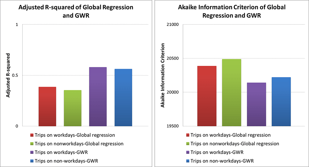
Fig. 3: Comparisons of explanatory power of Global regression and GWR.
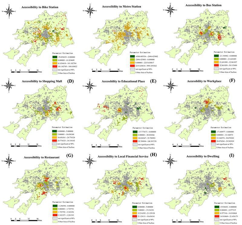
Fig. 4: Spatial distributions of local coefficients on working day and t-value with significance less than 90%.
Conclusions
Global Regression
GWR
The capacity and proximity of bike stations are positively correlated with bike usage.
Gravity-based accessibility to metro stations of bike stations may increase bike flow.
The bike stations nearby shopping malls, bus stations, restaurants, financial and educational places are also positively correlated with bike usage.
Population density has a statistically negative impact on bike usage.
The effects of built environment are divergent across the Suzhou region.
Most of the coefficient appears to have zero or negative value in the central areas of Suzhou (Old Town) while surrounding areas have modest built environment effect on bike flows.
The goodness of fit in the GWR is better than the global regression model.
Acknowledgements
This work was supported by Jiangsu Industrial Technology Research Institute and Research Institute of Future Cities at Xi’an Jiaotong-Liverpool University.
For more detailed information please contact our TUPA members below;
Chunliang Wu, [email protected]
Transportation data is of great importance for intelligent transportation system. Missing data problems are inevitable during data collection.
Challenges in existing imputation methods: potential useful information is not efficiently used in the modeling process; methods considering temporal correlation usually assuming that linear relationships exist between observed variables and latent variables; most techniques fail to measure the uncertainty.
This study introduces the use of a self-measuring multi-task Gaussian process (SM-MTGP) method for imputing missing data.
CONTRIBUTIONS
A SM-MTGP method is proposed to combine features from tasks and inputs to measure similarities jointly.
Dependencies of tasks and inputs are explored via covariance functions under SM-MTGP framework.
Correlations between responses are captured to provide additional information for enhancing imputation accuracy.
METHODOLOGY
Brief review of MTGP
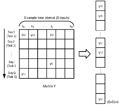
Assuming we have \(Q\) tasks and a set of observations \(Y = \left\{ {{y_{i1}},{y_{i2}}, \ldots {y_{iD}}} \right\}, i = 1, \ldots ,Q\), for each corresponding task at \(????\) distinct inputs, where \(????_{????????}\) is the response for \(????^{????ℎ}\) task given the input \(????_????\).
FIGURE 1 Vectorization of matrix Y
When the SM-MTGP model is introduced to the imputation of missing values of transfer passenger flow, the shared information of tasks is considered in terms of the temporal relatedness of various days. Transfer passenger flow over \(Q\) days can be treated as \(Q\) tasks, and the number of sampling time intervals \(D\) per day represents \(D\) distinct inputs. We define a matrix \(Y = \left\{ {{y_{ij}}} \right\}(i = 1,2,…,Q;j = 1,2,…D) \in Q \times D \), where \({{y_{ij}}}\) is number of transfer passengers for the \({i^{th}}\) day (task) on the \({j^{th}}\) time interval (input). By stacking the column vectors of \(Y \in Q \times D \), a \(Q \times D\) dimension vector \({\bf{y}} = vec(Y)\) is obtained (Figure 1).
The MTGP model of \({{\bf{\tilde y}}}\)can be described as Equation (1):
$${{\tilde y}_{ij}} = {m_{ij}} + \varepsilon ,\quad \varepsilon \sim N\left( {0,{\sigma ^2}} \right) \tag{1}$$ where \({m_{ij}}\) is the expected value of the element \({{\tilde y}_{ij}}\), and \(\varepsilon\) is an additive Gaussian noise with variance \({{\sigma ^2}}\).
$$m \sim N\left( {0,{\Sigma _Q} \otimes {\Sigma _D}} \right) \label{TGP} \tag{2}$$ $${\Sigma _Q} = K_Q^fG_Q^m, \quad{\Sigma _D} = K_D^fG_D^m \label{covariance matrix} \tag{3}$$ The covariance matrices \({\Sigma _Q}\) are defined as a product of kernel of days features (tasks) \(K_Q^f\) and the self-measuring kernel \(G_Q^m\), and \({\Sigma _D}\) are defined as a product of the kernel of time intervals features (inputs) \(K_D^f\) and self-measuring kernel \(G_D^m\).
$${K_Q^f} = k\left( {{y_i},{y_j}} \right) \in \mathbb{R}^{Q \times Q}, \quad {G_Q^m} = g\left( {{y_{i:}},{y_{j:}}} \right) \in \mathbb{R}^{Q \times Q} \tag{4}$$ $${K_D^f} = k\left( {{y_h},{y_l}} \right) \in \mathbb{R}^{D \times D}, \quad {G_D^m} = g\left( {{y_{:h}},{y_{:l}}} \right) \in \mathbb{R}^{D \times D} \tag{5}$$ where \(k\left( {{y_i},{y_j}} \right)\) and \(k\left( {{y_h},{y_l}} \right)\) indicate covariances of features of \({i^{th}}\) day and \({j^{th}}\) day, and covariances of features of \({h^{th}}\) time interval and \({l^{th}}\) time interval, respectively. Similarly, \(g\left( {{y_{i:}},{y_{j:}}} \right)\) and \(g\left( {{y_{:h}},{y_{:l}}} \right)\) measure covariances of self-measuring observations of \({i^{th}}\) day and \({j^{th}}\) day, and covariances of self-measuring observations of \({h^{th}}\) time interval and \({l^{th}}\) time interval.
By following the principle of MTGP, the joint distribution of \({\tilde Y}\) can be described as Equation (6), where \(\Phi = {\Sigma _Q} \otimes {\Sigma _D} + {\sigma ^2}{\bf{I}}\).
$$\int {p\left( {\tilde Y|M,0,{\sigma ^2}} \right)} p\left( {M|{\Sigma _Q},{\Sigma _D}} \right)dM = N\left( {{\bf{\tilde y}}|{\bf{0}},\Phi } \right) \tag{6}$$ Using a Gussian process framework given the observed number of transfer passengers, the unobserved passenger flows in \(Y\) can be derived by predictive equation (7). $$E[{{\tilde y}_{ab}}|{{{\bf{\tilde y}}}_{obs}},{\Sigma _Q},{\Sigma _D}] = \left( {{\Sigma _{{Q_a}}} \otimes {K_{{D_b}}}} \right)_{obs}^T\Phi _{obs}^{ – 1}{{{\bf{\tilde y}}}_{obs}} \tag{7}$$ where \({\Phi _{obs}} = {\bf{P}}\Phi {{\bf{P}}^T} \in \mathbb{R}^{M \times M} \) is a covariance matrix over the observed transfer passenger flows in \(Y\), \({{\Sigma _{{Q_a}}}}\) denotes \({a^{th}}\) column vector in \({\Sigma _Q}\), which measures the similarities between \({a^{th}}\) day and all the other days among \(Q\) days, and \({{K_{{D_b}}}}\) indicates \({b^{th}}\) column vector of \({K_D}\), which represents covariance between \({b^{th}}\) time interval and all the remaining time intervals of \(D\) samples.
EXPERIMENT
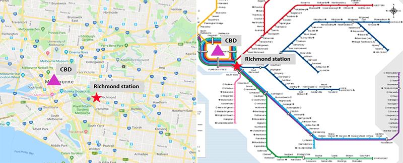
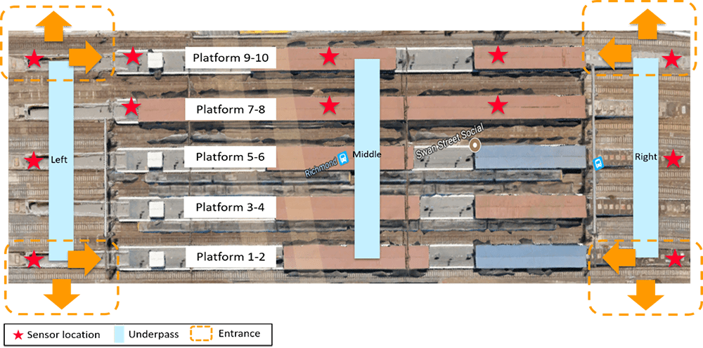
Data analysed includes 6-months of passenger flow data collected by WiFi sensors at Richmond railway station (Figure 2), Melbourne, Australia.
FIGURE 2 Map of location and train lines of Richmond station.
FIGURE 3 Map of 12 WiFi sensors distribution.
The deployed 12 sensors are distributed at platforms 7-10 and two sided underpasses (Figure 3).
IMPUTATION PERFORMANCE
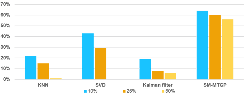
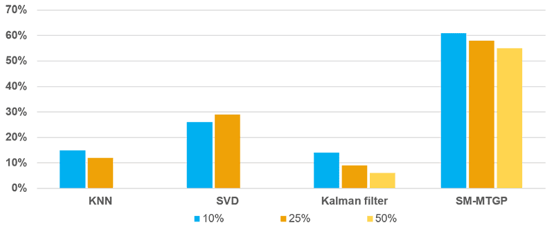
Figure 4 indicates the RMSE results of discrete missing pattern with various algorithms. The improvements in RMSE by SM-MTGP is around 60% for three different missing rates.
FIGURE 4 RMSE Results for Different Missing Ratios of Discrete missing data.
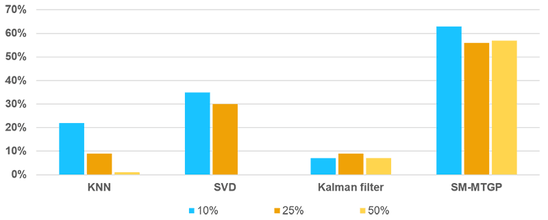
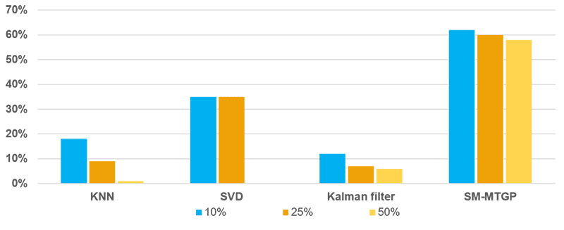
Three mixed missing patterns under different missing ratios are reported (Figure 5-7). The SM-MTGP method is still able to obtain better performance compared with all the other methods, leading to improvements in RMSE up to 60%.
FIGURE 5 RMSE Results for Different Missing Ratios of Mixed Missing Data
with One Random Day Missing.
FIGURE 6 RMSE Results for Different Missing Ratios of Mixed Missing Data
with Two Random Day Missing.
FIGURE 7 RMSE Results for Different Missing Ratios of Mixed Missing Data
with Four Random Day Missing.
CONCLUSIONS
Imputation accuracy can achieve around 60% improvement in RMSE in all the tested missing scenarios compared with the base model.
SM-MTGP significantly outperforms other methods under the large missing ratio.
On-going research on incorporating other features into this algorithm to make application on large-scale transit network and simplifying model computational complexity.
For more detailed information please contact our TUPA members below;
Wenhua Jiang, [email protected]
It’s not easy to pick up this background image for the post. It shows the Manhattan Peninsula, New York, and the sky reflects the buildings on the ground. This fantasy scene reminds me the complex relationship between space and time, which closely related to the topic of this article: Spatiotemporal forecasting of traffic by using 3d convolutional neural networks.
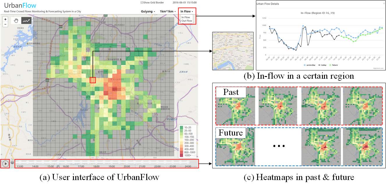
On December 31, 2014, a deadly stampede occurred in Shanghai, near Chen Yi Square on the Bund, where around 300,000 people had gathered for the new year celebration. 36 people were killed and there were 49 injured, 13 seriously (Wikipedia). From the follow-up reports, it can be known that Tencent’s user online information has roughly detected that the traffic in the area was too dense. So data from social media and cell phone signal can infer the regional crowd density. If the corresponding predictions and analysis can be made, such tragedies will not happen.
Traffic forecasting has been studied for decades. There are many outcomes of models and theories. For the regional prediction, it’s a prevalent way to split the research area into grids and analysis them by computer vision models. Each square in the girds just like the pixel in an image.
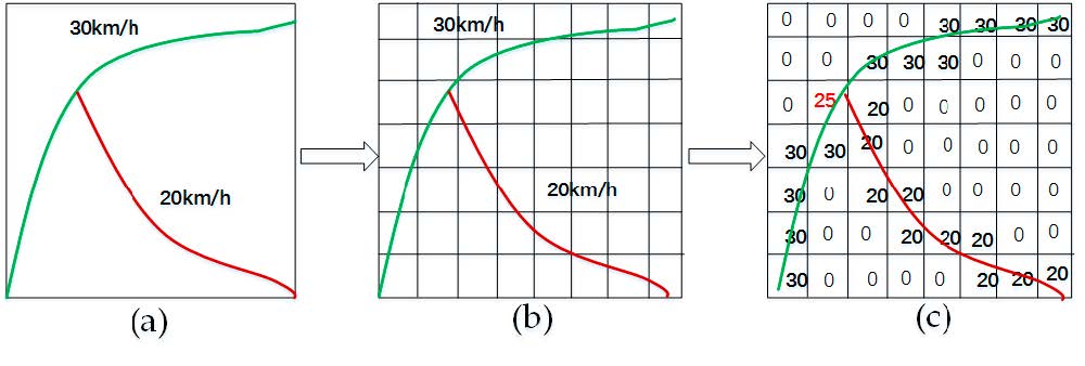
Zhang (2016) presented the classic Deep-ST model. It treats the research area as image and the predicted result combined with the convolutional models from different periods. However, the convert not only limited to traffic volume. The vehicle speed can also be transformed into images. The images below shows the traffic speed representation in a small-scale transportation network (Yu, et al 2017).
With the development of computer vision, deeper neural networks like ResNet has been presented recently. Zhang (2017) also upgraded the DeepST to ST-ResNet with ResNet models. However, the convolutional kernel in these models only focuses on spatial relations, not for a spatiotemporal space. It’s been proved that 3D Convolutional Networks can learn the spatiotemporal features (Tran 2015). But these improvements only appears in video related studies like behavior detection, human action detection, etc. So in this post, we will see the application of 3D ConvNets on traffic problems.
Convolutional operations
There are some different operations with the convolutional kernel in hidden layers. The following diagrams show the 2D convolutional operation with padding and dilation (Dumoulin and Visin, 2016 ). It’s different in 3D, but the ideas are same.
With the 3D convolutional operation, the kernel shape is 3 dimensional and it moves in 3 directions. Just like the animation below. For the transportation problems, the directions are latitude, longitude and time. In the model part, we also used padding and dilation with 3D kernels.
Data and Model
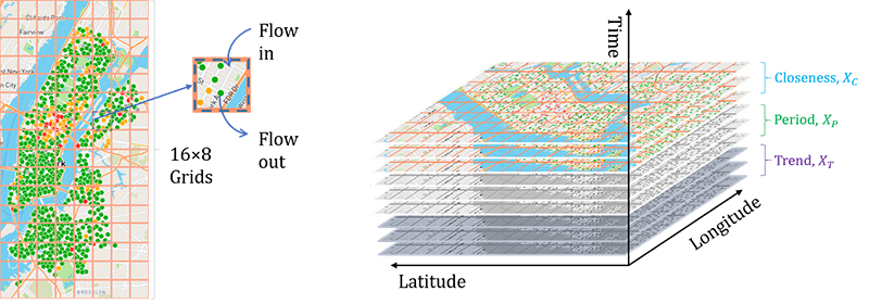
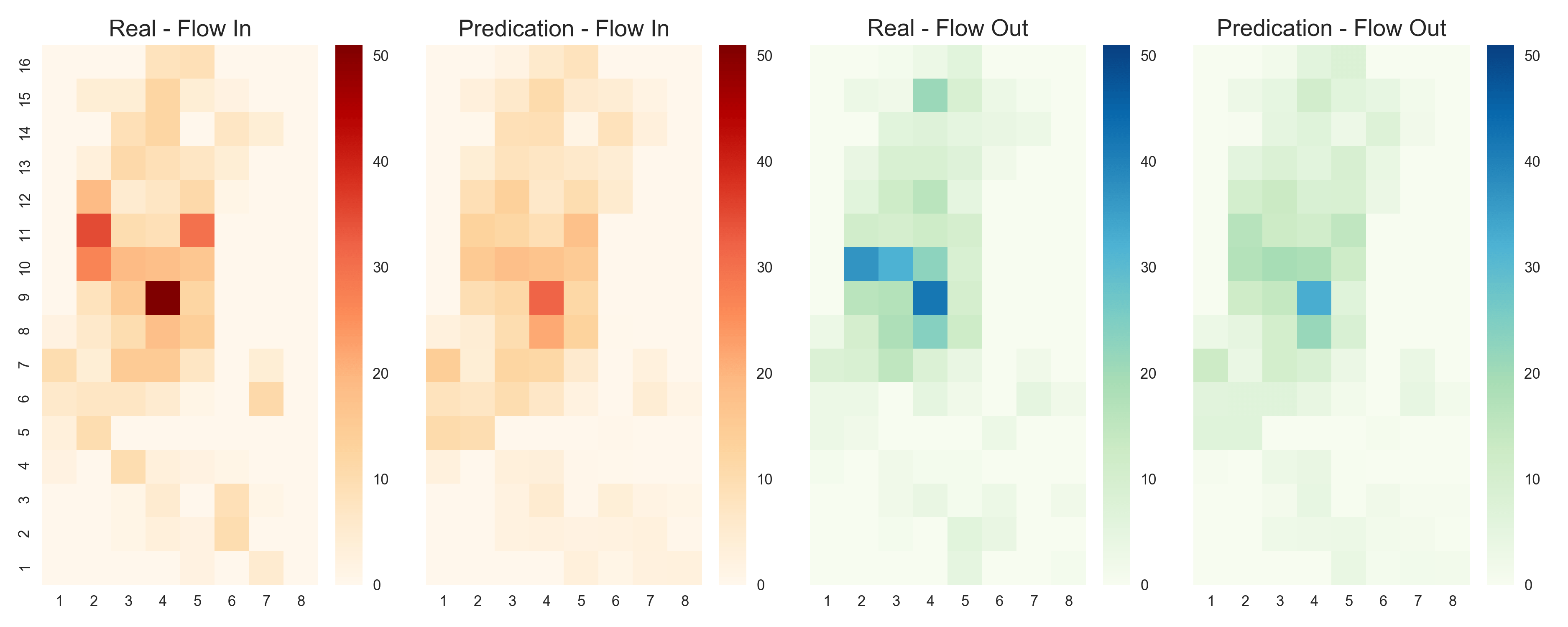
We take the bike sharing data in New York (BikeNYC) from the DeepST paper as an example here. Every circle stands for a station and the color means the number of bikes in dock. The research area is split into 16*8 grids, each square has in and out flow at a particular moment. The in and out flow are numbers of return and borrow bikes in the corresponding region.
The input is a time sequence from the time level of closeness, period and trend. They stand for the different extract frequency from raw data. If stack them together, the input shape would be X168. The X is the number of timesteps.
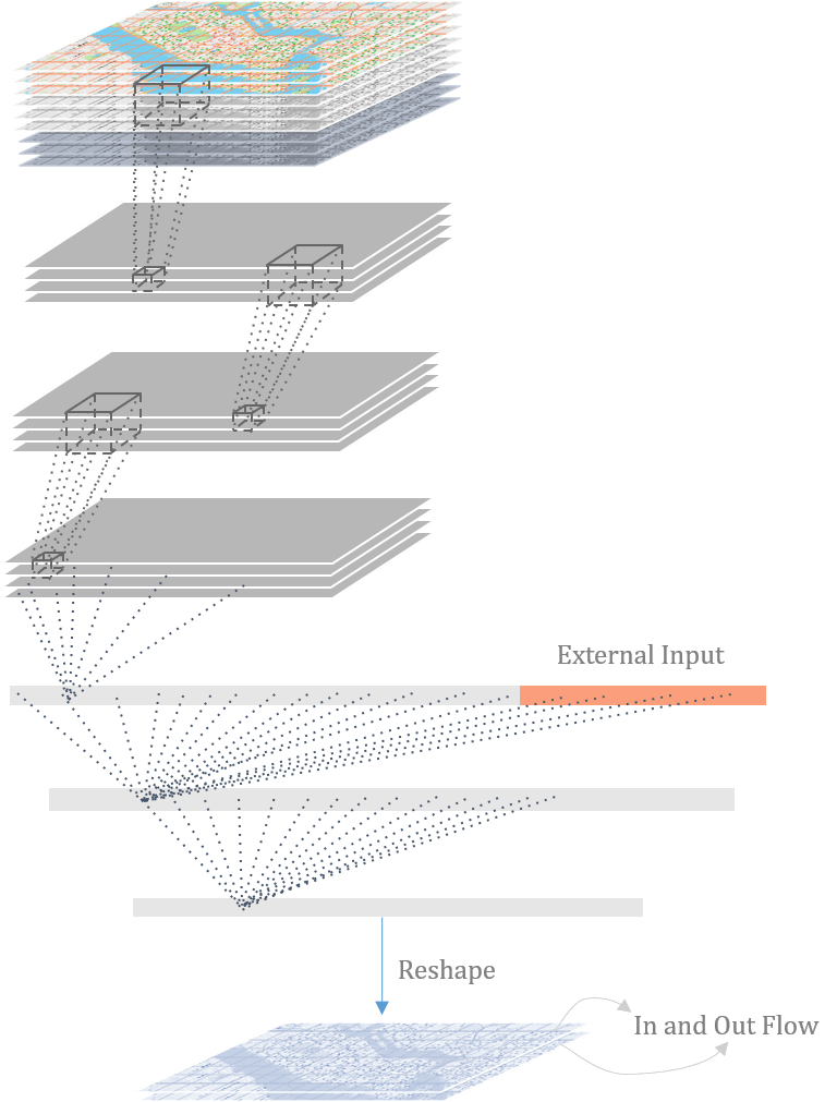
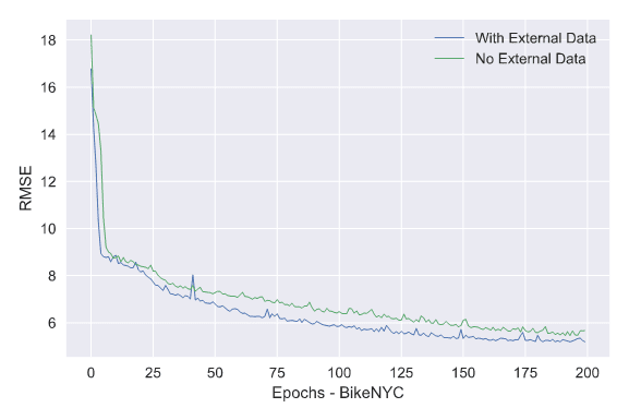
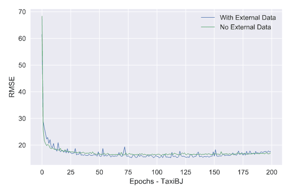
The model has three 3D convolutional layers and the flatten layer combines the external data like weather and holidays.
Experiments
I used Pytorch this time. The windows version just came out last month. It provides a lot of API and very easy to build a custom model structure. The author of ST-ResNet has opened his code, so we can reuse the dataset from Github.
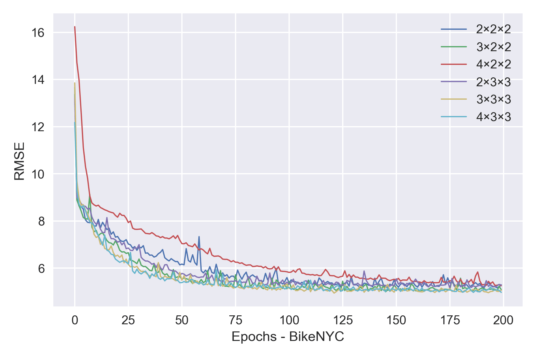
To get the best kernel size, we take different combinations for training test. It turns out that 3*3*3 is also the optimal option for transportation data just like other papers have pointed out in some behavior detection tasks.
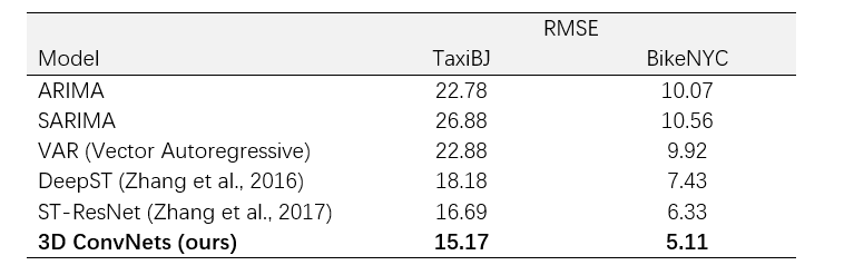
Although the model is much simpler than Deep-ST or ST-ResNet, it still achieved the best performance on BikeNYC and TaxiBJ datasets.
Visualization
Firstly, I have tried the Matplotlib in Python. The outcomes are good but they are static and not appropriate for the webpage. So I chose d3.js to draw the diagram from scratch. (The style with CSS and SVG tags is incompatible with this blog responsive CSS sheet. So I just give up displaying it on this page. Here is the gif version, simple and straightforward.)
Zhang, J., Zheng, Y., Qi, D., Li, R., & Yi, X. (2016, October). DNN-based prediction model for spatio-temporal data. In Proceedings of the 24th ACM SIGSPATIAL International Conference on Advances in Geographic Information Systems (p. 92). ACM.
Zhang, J., Zheng, Y., & Qi, D. (2017, February). Deep Spatio-Temporal Residual Networks for Citywide Crowd Flows Prediction. In AAAI (pp. 1655-1661).
Tran, D., Bourdev, L., Fergus, R., Torresani, L., & Paluri, M. (2015, December). Learning spatiotemporal features with 3d convolutional networks. In Computer Vision (ICCV), 2015 IEEE International Conference on (pp. 4489-4497). IEEE.
Vincent Dumoulin, Francesco Visin – A guide to convolution arithmetic for deep learning