The lane change behaviour is not only impacted by the blockage but also the surrounding traffic.  The combination of these two impacts determines the subject vehicle lane change execution behaviour: i.e. to either Continue lane change execution or Not Continue lane change execution.

We developed the lane change execution model based on the model framework, followed by the lane change execution model (LCEM) calibration.  The lane change execution behaviour of PC is different from that of HV, it is worth exploring the LCEM for PC and HV separately. Based on the results of LCEM and analysis of the lane change execution characteristics of PC and HV, the LCEM for PC and HV are established and parameters are estimated accordingly.

Lane Change Execution Model Evaluation with Micro-Simulation Outcomes

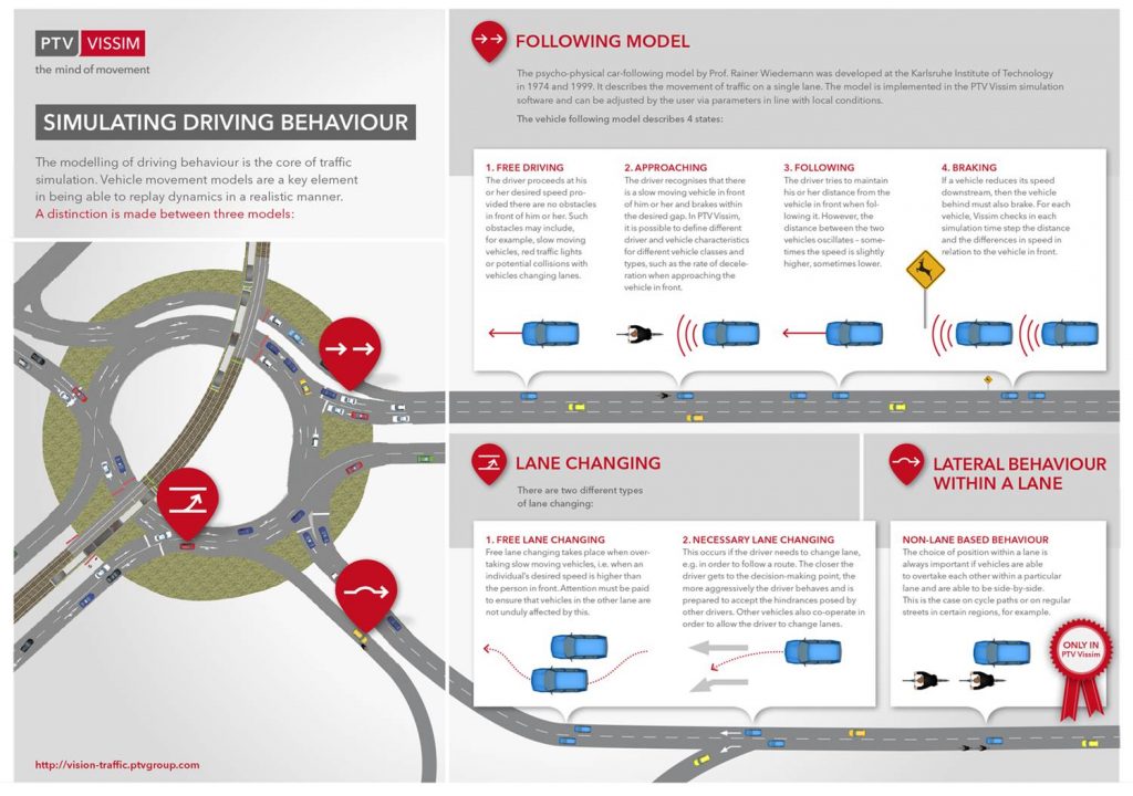
Microscopic traffic simulation is an efficient and widely-used tool for analyzing the performance  of roadways on traffic, safety and the transportation system (Young, Sobhani et al. 2014).  The core of a simulation model is a set of mathematical algorithms that evaluate the motion of each vehicle on a second-by-second basis as it interacts with the road network, the traffic control system and the surrounding traffic environment.  A lane-changing model is incorporated as one of the basic driver behaviour interaction in the microscopic traffic simulations based on different algorithms.  Two major simulation models (VISSIM (2012)and AIMSUN (2012)) outputs of lane change processes are analyzed in this section.

• VISSIM

To assure a model reproduces real-world traffic conditions reasonably well, the simulation parameters have been calibrated using the data collected by the same camera. Headway is used as an indicator to adjust the parameter values.  When the Mann Whitney U test shows the distributions of headway from simulation and observation are comparable, the calibration process is completed. It is noted that after the calibration completed, VISSIM still provides the fixed value for lane change duration due to lack of lane change execution models integrated.

The output from Vissim shows that the duration of lane change is a fixed value.  For the passenger cars (PC), the lane change duration is 2.2s; and for the heavy vehicles (HV), the duration is 2.4s.  However, from the observed data collected in this study the lane change durations vary from 1s to 6.8s for both vehicle types.  The distributions of lane change duration from the observed data for PC and HV are shown.

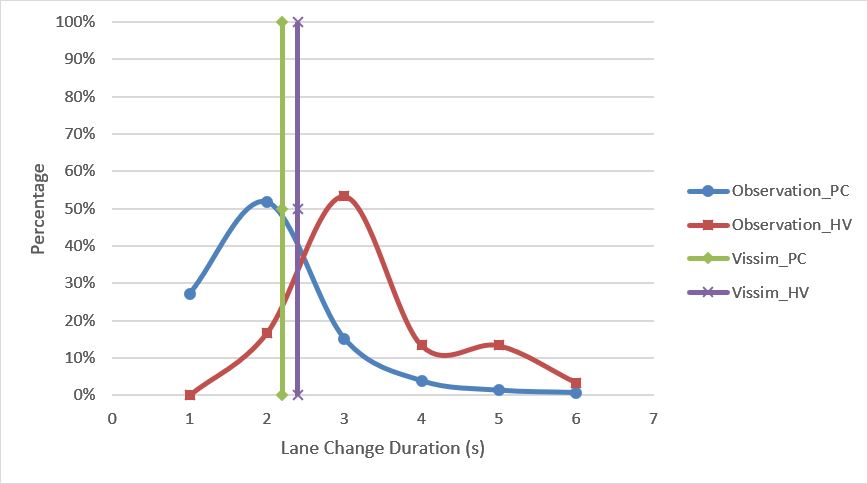
Distributions of Lane Change Duration of PC and HV from Observation

 In terms of the lane change trajectory analysis, Vissim provides the lane change start and end locations which indicate the lane change trajectory in the longitudinal direction.  For passenger cars, the lane change length from Vissim ranges from 1.6m to 32.4m, while the observation of the lane change length ranges from 19.6m to 76.3m.  Figure 8-2 shows the distributions of the lane change length in longitudinal direction for passenger cars between Vissim output and observation. For heavy vehicles, the lane change length from Vissim ranges from 4.1m to 28.7m, while the observation of the lane change length ranges from 40.3m to 96.7m. Figure 8-3 shows the distributions of the lane change length in longitudinal direction for heavy vehicles between Vissim output and observation. The result implies that the lane change trajectory Vissim generates is much different from the real-life lane change trajectory for both passenger cars and heavy vehicles.

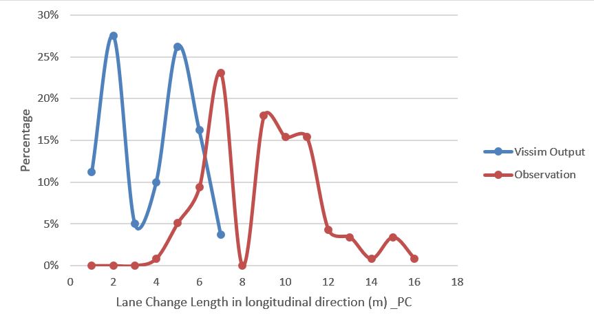
Distributions of Lane Change Length in Longitudinal Direction of PC

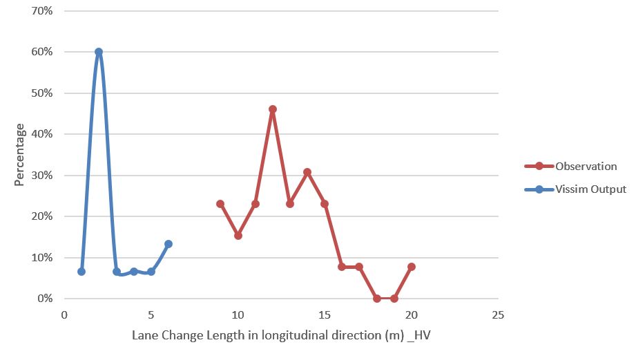
Distributions of Lane Change Length in Longitudinal Direction of HV

• AIMSUN

Figure shows the distributions of travel time during the blocked section for the passenger cars.  The travel time of passenger car from AIMSUN ranges from 2.6s to 16.8s, while the travel time of passenger car from observation ranges from 7s to 21.2s. It can be seen that the travel time is generally smaller than the observed travel time. Especially the minimal travel time from AIMSUN output is 2.6s which is 4.4s smaller than the minimal travel time of observations. It is not realistic for a PC to complete 140m in 2.6s.

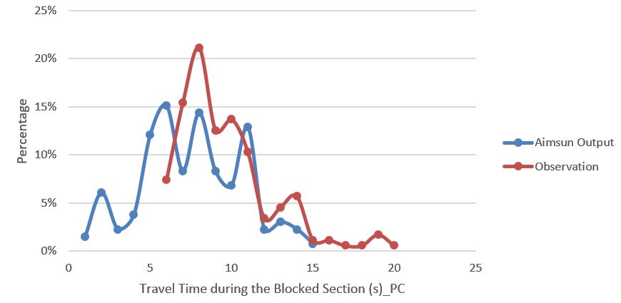
Distributions of Travel Time of PC during the Blocked Section

Figure shows the distributions of travel time during the blocked section for heavy vehicles. The travel time of heavy vehicle extracted from AIMSUN ranges from 13.4s to 16s, while the travel time of passenger car from observation ranges from 9s to 21.6s.  It can be seen the travel time from observations for HV has a larger range while the travel time from AIMSUN output is clustered in a certain range, which means it does not reflect the observation well.

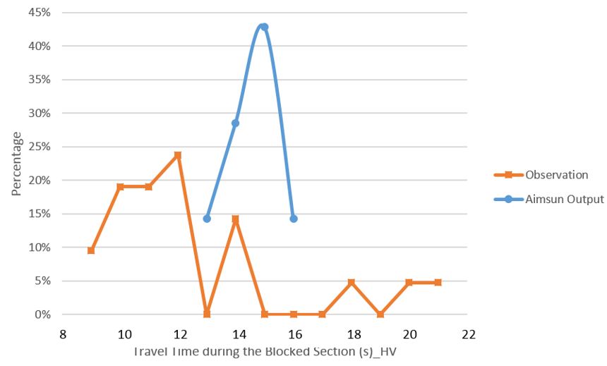
Distributions of Travel Time of HV during the Blocked Section

The results imply that the AIMSUN output differs from the observed data on lane change execution collected for this study, especially for the heavy vehicles.

Evaluation of Lane Change Execution Model

The lane change execution model is applied on the existing simulation outputs. This study assesses the results from lane change execution model and the real-life data to see the improvement of the model to the simulation output.

To apply the LCEM on the simulation output, the traffic output data need to be extracted from Vissim, identifying the subject vehicles and direct surrounding vehicles and recording the each vehicle traffic information in every 0.1s. A Matlab program is developed to apply the LCEM using the basic vehicle information from Vissim to predict the lane change behaviour. The result of lane change execution prediction (Continue Lane Change or Not Continue Lane Change) is thus used to identify the lane change execution durations.

The original output from Vissim shows that the duration of lane change is a fixed value, which is 2.2s for passenger cars.  The original simulation output is apparently not fitting the distribution of the lane change duration observation.  While applying the lane change execution model on Vissim, the lane change duration distribution is fitting the duration distribution of observations much better.

Figure shows the comparison of passenger car lane change duration distribution between the outputs applied the execution model, the real-life observed data and the outputs from simulations. The lane change duration of PC in Vissim is 2.2s and 0s in Aimsun. The comparison indicates that the lane change execution model is able to improve the simulation outputs to fit the real life lane change behaviour better for the passenger cars.

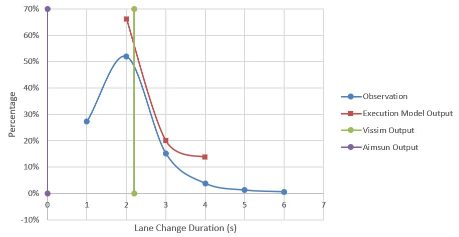
Comparison of Lane Change Duration Outputs for PC

The limitation of this work is all durations of the outputs are larger than 2.2s which is the fixed value provided from Vissim.  It can be seen that the range of 2~3s has very high portion in the model output compared to other duration ranges. The reason could be that it also includes the lane change durations which are smaller than 2.2s. This could be a good part of the future work to improve the current simulations.

Figure shows the comparison of heavy vehicle lane change duration distribution between the outputs applied the execution model, the real-life observed data and the outputs from simulations.  The lane change duration of HV in Vissim is 2.4s and 0s in Aimsun. The distribution of HV lane change duration is not as good as the distribution of PC lane change duration which fits the observed data better. However the trend of lane change duration is close to the observations than the outputs from the current traffic simulations. The result also indicates that employing the lane change execution model for HV would obtain the outputs closer to the real life lane change behaviour.

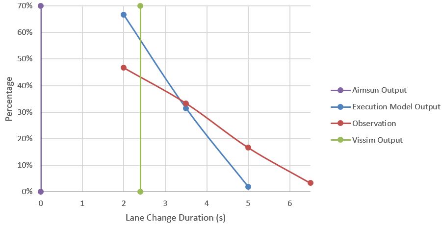
Comparison of Lane Change Duration Outputs for HV

Similar to the limitation for PC, the high portion of 2.5~3s of HV lane change duration could be caused by the fixed value of 2.4s which are extracted from Vissim.  Moreover, the size of observed data samples also could be a limitation of this work. The further work will need to collect more data for HV in different location.

Part One: Bike-share in China and Suzhou

Bike-share systems (BSs) are generally believed to be a sustainable and healthy transport mode and have the potential to enhance public transport by offering a last-mile service. The merging of BSs worldwide has been a relatively new trend. By the end of 2016, 1,286 BSs had been deployed worldwide, among which, the largest and fastest increasing BSs market is in China -by the end of 2016, China had established 430 BSs with a bike fleet of 1.9 million, making it the largest BSs market in the world, followed by Italy and USA, as shown in the following figure (note that the uprising dockless bike-share systems like Mobike are not included).

Top 10 bike-share system countries (by the end of 2016)

As for Suzhou Public Bike System (SPBS), it is a third generation bike-share system located in Suzhou – a major city (2,743 km2, 6.7 million population) located in East China. SPBS is operated by a private company Youon, under the supervision of Suzhou Urban Management Bureau (SUMB) – a local bike-share administration authority. It was first launched on August 30, 2010, with only 11 stations and 200 bikes. Currently, over 2,200 SPBS stations and 41,000 fleets are distributed all over the city. The average daily ridership of SPBS is more than 0.2 million in 2016, namely each SPBS bike used 4.7 times/day. SPBS contributes 0.32% of the overall transport modes.

Distribution of SPBS stations in Suzhou

Notes:
1. drag and scroll a mouse wheel to zoom in and out to search different areas
2. color:
Red circle – areas with stations >100
Yellow circle – areas with stations between 10 and 100
Green circle – areas with stations < 10

Access to SPBS was initially available to people who registered for a membership card. In 2016, Youon upgraded the system to allow smart phone access, so users can register, check in and out and receive information through an APP without a card. To some extent, it makes SPBS a third-half generation BSs.

For SPBS charging policy, the deposit is USD 30 for card registrations and free for APP registrations. The first hour’s ride is always free followed by USD 0.15 /h. No extra subscription fees or membership fees are needed. The financial requirements to gain access to the system are easy since cycling users are encouraged and subsided by government. Compared to western bike-share systems, great advantages could be seen in SPBS. See the following table.

Part Two: what do trip data tell us about SPBS

By using dataset provided by SUMB, we are able to get access to over 30 million SPBS trip records, which covers all 2,256 stations in Suzhou from June 1, 2016 to May 31, 2017. By analyzing this big data, tempo-spatial distribution, users’ characteristics and behaviors could be revealed.

Usage of SPBS in a random working day

Firstly, by dividing the picking up and returning activities, we could see how SPBS usage changes in a random working day in 24 hours in a city-scale. Two peak hours from 7 to 8 am and from 5 to 6 pm could be observed with unbalanced spatial distribution—— more pick-up activities could be observed in certain areas while other areas with more returning activities in peak hours.

Notes:
1. Every dote indicates a SPBS station
2. Different color means different numbers
3. Time can be seen in top left

SPBS trips dynamic assignment in a given weekday in a whole day

Since cycling in all SPBS stations can be tracked, a stations matrix is built up so that all the cycling trips could be assigned to existing road network. This following video shows how SPBS trips are assigned to road network in a random working day. A complete road network with all the public bike stations is built up and the assignment process is optimized so that cycling trips only exist in urban streets rather than expressways and freeways. Densest trips could be seen in roads in SIP, SND.

[jwp-video n=”1″]

Notes:
1. line width indicates trips numbers, thicker lines mean more bike trips
2. Time could be seen in bottom right

Average travel time by age and gender

Profiling method is used to analyze users characterizes. In the following two figures, trips from Jun 2016 to Jan 2017 are aggregated and trip time is distributed monthly in terms of different groups (by age and gender). It turns out that
young group (18-34 years old) and male group favor public bike more than other groups, while 5 min is the most popular trip time.

Notes:
1. legend is on the right, four age groups are divided
2. move the mouse on the figure and details would show out
3. Y-axis is ratio and X-axis is trip time.

Weekly trip frequency distribution by age

The following figure displays the weekly frequency of SPBS users in different age groups. Most people travel less than two times in one week – and younger the user are, more often they use public bikes.

Notes:
1. Legend is on the right, four age groups are divided
2. Move the mouse on the figure and details would show out

Year-trip distribution by age

This visualization shows that the total number of trip times of each month in different age groups from June 2016 to May 2017. People aged between 18 and 54 are the major user group of public shared bikes in Suzhou. In addition, the usage frequency of SPBS varies in different quarters. It indicates that the temperature and other environmental factors have a significant impact the usage of shared bikes. – for instance, in Jan and Feb (normally Spring Festival holidays), SPBS usage was greatly fluctuated and influenced.

Tips:
1. Legend is on the right, four age groups are divided
2. Move the mouse in each month line to see the detailed information

Access methods and users’ preference in a year

From 2016, users are able to get access to public bike system by scanning QR code through smart phone, which offers a convenient way to use public bike system. In this visualization, total trips grouped by two access methods (traditional smart card and QR) are given.
Big jump of QR users clearly indicates users’ preference on convenience.

Notes:
1. Legend is on the top right
2. Drag the bar at the bottom left and right to move horizontally to look close a chosen span

Access methods and users’ preference in a week

Two types of users (QR users and smart card users) are indicated and compared in a random working day in this figure. Interestingly, more people use smart card in the morning peak hour while scanning QR is more popular in night peak hour.

Notes:
1. Legend is on the right
2. Press play to watch how different access methods works in each day in a week

Part Three: What happened when Metro meets Bike-share

Metro Line 4 (known as the M4) is the third metro line operating in Suzhou which runs from the north (Xiangcheng District) to the south (Wuzhong District) crossing through the central area. It was opened on 15th April 2017 while the SPBS dataset spanned from June 1, 2016, to May 31, 2017, namely, trip dataset offers time windows to measure changes of SPBS before and after the metro opened. We selected 84 SPBS stations alongside M4 to see how metro influenced SPBS usage.

Changing rate of trips caused by M4

Ridership is found to soar greatly after the M4 was introduced, as the city-level SPBS trips increased from 3.6 million to 5.34 million at a rate of 148.1% from March to May. Not surprisingly, alongside M4, the chosen stations witnessed greater increase at a rate of 190% as can be seen in following figure.

Note that larger increase in weekend trips compared to weekday trips at both city-level and selected stations means the new metro may have triggered more leisure cycling than commuting cycling.

Interestingly, the average travelling times declined from 17.2 mins to 15.9 mins at the selected stations while increased in a city-level. This is logical proof of how transit and bike-share combine. In SPBS stations accompanying the M4, cycling time was reduced because an interchange has been introduced, in the form of the metro, into what was once a total cycling trip.

Notes:
1. Legend is on the top
2. The numbers above the bar indicates the changing rate of cycling times

Ridership change alongside M4

The following figure shows how trip number changes when M4 is introduced. Basically, most of the stations witnessed a increasing rate after M4 operated.

Notes:
Blue bars mean increasing rate of trip numbers in particular stations while the red means decrease. The higher, the greater change

Patterns change caused by M4

By analyzing and clustering trips in stations alongside M4 by k-means algorithm, two major types of trip patterns are revealed. They are called “balanced pattern” and “imbalanced pattern”. If a station has similar borrowing and returning number of bikes in most of the time, they are defined as “balanced pattern”, otherwise, they behave “imbalanced pattern”.

A typical balanced M4 station (Beisita)

Notes:
1. Red bar indicates returning bikes while blue indicates borrowing, they are almost the same
2. X-axis is time vector and Y-axis is returning/borrowing times

A typical imbalanced M4 station (Huolidao)

The pre- and post- patterns of trips were then compared since correspondent type categories are already set, see the following Figure. A changing pattern from balanced to imbalanced (higher number of arrivals in the morning and higher number of departures in the evening) is commonly observed.

Notes:
1. Red bar indicates returning bikes while blue indicates borrowing, they are almost the same
2. X-axis is time vector and Y-axis is returning/borrowing times

Patterns changed due to M4

Tips:
1. Left figure is station patterns before M4, right figure is how it changed after M4
2. Blue circle indicates SPBS stations with balanced patterns while red indicates imbalanced ones

Some interpretation and possible reasons behind

A changing pattern from balanced to imbalanced (higher arrivals in the morning and higher departures in the evening) along with increasing trips might be understandable in residential areas since people tend to cycle to “arrive” at metro stations and “depart” from there. However, this also happened in mixed-use areas, where it was assumed people would have “arrived” on the metro and used shared bikes to “depart” to their work places, resulting in high borrowings (departure). To the contrary and beyond expectation, the result of post-M4 clustering analysis suggests higher arrivals occur in mixed-use areas within core urban areas.

This phenomenon might be interpreted as more people cycling to the metro interchange from their homes rather than cycling to work places from the metro during the morning peak and vice versa in the evening, as seen in following Figure . In other words, the SPBS mainly serves as “first-mile” in the morning and “last-mile” in the evening on working days. Abundant, convenient interchanges available in core urban areas might be one of the reasons. Another reason might be the issue of rebalancing bikes at stations, returning bikes and the amount of walking. For example, when a traveler departs from a metro station and has to walk a while to rent a shared bike, he has to take the risk that the BSs station might be empty, and he has to walk further to reach another station.

Users changed due to M4

Three stations were selected to further investigate both the trip and user changes in a micro perspective. These three cases are chosen since they are in different yet typical land use patterns.

Huoli Dao station (ID 5034) is located among a large residential block in northern Suzhou, a relatively remote area right next to an entrance of an M4 station. The surrounding land use is mainly residential. After the M4 began operation, more than 900 new cyclists appeared while 368 users disappeared in almost a month. It is hypothesized that while some former users turned to the metro directly, most of the new users were attracted to the M4 by using shared bikes.

Tips:
1. blue circle indicates SPBS stations with balanced patterns while red indicates imbalanced ones
2. left figure is before M4, right figure is after M4
3 new users: new (active) BSs users.
casual users: active BSs users become casual users.
disappeared users: former BSs users have no usage records any more, which means they have stopped using the BSs

The International Education Center station (ID 2306) locates among a large block of education facilities. The land use is solely for education. After introduction M4, some former users abandoned the SPBS while slightly more new users began to use shared bikes (584 vs 705) as shown in Figure 15. This indicates that the M4 has triggered and attracted a growing number of new SPBS users.

Le Qiao station (ID 87) locates in the heart of Suzhou, the center of the old town comprising mixed land use and a commercial center nearby. Note that it is located near the M1 that began operation 4 years earlier than the M4. The shift in users is particularly interesting at this station, where over 1,200 users abandoned the SPBS while almost 1,000 new users emerged once the M4 began operation. The absolute numbers from both sides are shown in following figure. Maybe the new metro (M4) substituted cycling in core urban areas as Martin and Shaheen (2014) described in two cases in the USA.

Authored by Wang, Chen and Kim

The bike-sharing service has brought many conveniences to citizens and served as an effective supplement to mass transit system. For docked bike-sharing service, each docking station has the fixed spots to store bikes and stations could be empty or saturated at some time. Bike-sharing operators would redistribute bikes between stations by trucks according to their experiences. It is ineffective for the operation and inconvenient for users to access this service smoothly. There are many studies on short-term forecasting in transportation, such as traffic flow, traffic congestion, traffic speed, passenger flow and more. However, their applications in the field of bike-sharing still remain blank. This paper mainly focuses on the short-term forecasting for docking station usage in a case of Suzhou, China. The widely used methodologies in forecasting are reviewed and compared. After that, two latest and highly efficient models, LSTM and GRU, are adopted to predict the short-term available number of bikes in docking stations with one-month historical data. RF is used to be compered as a benchmark. The predicted results show that LSTM and GRU which derive from RNN and Random Forest achieve good performance with acceptable error and comparative accuracies.  Random forest is more advantageous in terms of training time while LSTM with various structures can predict better for long term.  The maximum difference between the real data and predicted value is only 1 or 2 bikes, which supports the developed models are practically ready to use.

FIGURE 2 Locations of the stations.

LSTM

The Long short-term memory neural networks (LSTM) is a special kind of recurrent neural networks for the time series prediction (28). As shown in the Figure 4 (a), the LSTM cell can hold and update a state during the training process. Thus, the model makes a prediction with the previous learning experience. The mathematical expressions can be denoted as

where  is the current step,  is the input,  is the output,  is the weight matrix,  is the bias. , ,  and  are intermediate variables, which decide to remember or forget the input data (29).

Two LSTM layers are used in this paper and the output layer would make a final regression results. Figure 4 (b) shows basic structure of the model as well as the running steps of the LSTM cells. When the continuous input values flow in the LSTM cell, it will unfold and handle these values by sequence as figure 4 (c). After the last one is finished, the cell would make an output result for the next layer.

FIGURE 4 Description of the LSTM model.

GRU

Gated Recurrent Unit (GRU) was introduced in 2014 (30). It’s an improved recurrent neural network based on LSTM. It merges the input part and forgetting part together so the number of the gates from 4 becomes 3. As a result, GRU saves more computational resources than LSTM with similar performance. To compare the difference between LSTM and GRU, we use same network structure as LSTM in figure 3 (b). The main expressions can be indicated by following formulas (29).

The article used LSTM, GRU and Random Forest with a different time interval and sequence length to predict the number of available bikes. A laptop (Windows 10, 16GB RAM, Intel i7-4720HQ, GeForce GTX 960M) completed the whole training tasks. The LSTM and GRU run on top of Keras (31) and Tensorflow (32)with GPU. For the random forest part, it is coded and run with Scikit-learn (33) and CPU.

The time interval only has three different levels: 1min, 5mins, and 10mins. Also, the sequence length has four different levels: 5, 10, 20, and 30. As a result, the lines in the graphs are not smooth but broken lines. The main features of these graphs are listed as follows.

• The MSE of RF is very good when the time interval is short but with the increase of the time interval, RF gets worse performance than other two. The memory unit in the RNN may help with long interval sequence;
• Generally, the results are quite similar with these three models. However, the blue line always higher than others in the graph of GRU and Random Forest, which means station 628 get worse results in those two models. Since 628 station has the larger usage amount, the variation may be higher than others;
• All lines get higher with the increase of the time interval. There are two potential reasons may cause this problem. One is that forecasting long time interval is harder. The other one is that the sample size is dramatically decreased when expanding the interval so that the accuracy is affected;
• Different sequence lengths do not change much performance of models but sequence lengths affect the results gently and the longer one leads to a better performance in most cases.

• LSTM, GRU and Random Forest are all following the trends very well. The difference between the real data and predicted data is less than 1 or 2 bikes. It is good enough to help to develop the bike-sharing management based on these predictions;
• The accuracies between the three predictions are very comparative;
• LSTM and GRU get similar trends in most of the cases because they might have similar model structures;
• When the time interval is short, random forest gets a better performance;
• By increasing the sequence length, the fluctuation of three predictions is

A big achievement on research!

Monash university, Institute of Advanced Vehicle technology and JITRI secured research funding of 4 million RMB( AU$ 760,000). The project title is Green Travel Models in Smart Cities: Coordination studies and Integration Platform Project.

The research is led by Dr. Inhi Kim, Prof. Terry Liu from SEU and Prof. Yifan Dai from THU.

This 3 year project, Monash is planning to recruit 4 phd candidates doing research on a variety of sub topics. I look forward to working on this project and making a great impact on traffic problems.

Subtopics are as follows;

1. Behavior analysis and demand forecasting based on multi-modal green travel
2. System optimization and resource allocation based on multi-modal green travel
3. Traffic control and demand management based on multi-modal green travel
4. induced travel based on traffic big data
5. Key technologies of cooperative vehicle-infrastructure systems.

A gated community in Shanghai

Chinese leadership under Xi Jinping is keen to improve traffic congestion in a variety of ways. Among pledges to create greener cities with more public transport, the ruling contained the apparently throwaway line that no more enclosed residential compounds will be built in principle and existing residential and corporate compounds will gradually open up so the interior roads can be put into public use. This would save land and help reallocate transport networks.

Our research team is now closely working with a Suzhou local company, CCDI to develop the index to evaluate the impact after implementing this program in China.

We developed a Wechat embedded application for helping police officers in China reduce their work load in issuing illegal parking tickets on site.

The application is designed for public to take a photo of the plate number of the illegal parking vehicle then simultaneously stores information such as the plate number, location, time, and a type of the car in our server. Based on threshold of  the location (10 m radius)and the time (for 30 min), the illegal parking ticket will be issued automatically to the driver.

The data will also be displayed on an electronic map of the city so that police officers can identify which street or area is problematic most.

This work is proudly done by our 2015 cohort student, Bo Wang.

Version 2 (09/07/2016)

Read more

Photo from Nash&Franciskato

Road rage is aggressive or angry behavior by a driver of an automobile or other road vehicle. Such behavior might include rude gestures, verbal insults, deliberately driving in an unsafe or threatening manner, or making threats. Road rage can lead to altercations, assaults, and collisions that result in injuries and even deaths. It can be thought of as an extreme case of aggressive driving.

Based on the characteristics, we analyse the road rage behaviours and suggest the control method.

A potential in ITS application to predict urban railway level crossing delays

The Victorian government has embarked on an eight year program to grade separate 50 level crossings around metropolitan Melbourne at an estimated cost of $AUD 5 to 6 B. A primary motivation of this program is to reduce delays to private motorists, freight vehicles and public transport services. As is common in an urban context, the existing level crossings are protected by boom barriers that control road traffic movements to ensure safe rail operation. Some of those crossings are effectively closed to traffic for up to three quarters of the peak hour. While this extensive capital works program will reduce delays at those locations, around 125 level crossings will be left untreated by the current grade separation project. This research examines the potential for Intelligent Transport Systems to reduce delays at urban railway level crossings. The characteristics of the current control system are examined to identify factors that contribute to delays to road users and a simulation model is used to model how ITS technology could be used reduce crossing closure times. The model highlights the value of improved train speed data and more accurate data on whether a particular train is to stop at a station adjacent to the crossing or run express through the level crossing.

The program: structure – 9 main areas, 5 year program with funding ~$5M

Rail crossing removal is NOT justified  – using existing benefit estimation methods

Source:  Nguyen, N, Currie G De Gruyter C Young W (2016 submission) ‘A New Method to Estimate the Aggregate Impacts of At-Grade Rail Crossing Impacts on Network Traffic Flow ’  Journal of Transport Geography

Impact of Removing ALL xings

Results in:

• 0.1% reduction in congested links
• 1.7% reduction in no. of severely congested road links
• 0.3% reduction in travel time

Study Flow

Hourly boarding and alighting passengers

Modeling Process

Platform density

Stair density

Waiting area LOS

This project was completed by KNU and Monash collaboration